This tutorial provides an overview of stress and strain in an engineering context.
Stress
At a basic level we define:
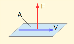
Normal stress σ in a material as σ = F/A where F is the normal force applied on area A
Shear stress τ in a material as τ = V/A where V is the tangential shearing force applied on area A
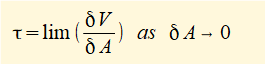
At a macro level these definitions of stress can be applied in situations where stresses are uniform over a large area, for example a steel bar in pure tension or compression. However, in many situations consideration of stress on a micro level is necessary and definitions are based on limits over a small element of area δA:
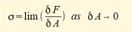
The unit for stress (σ and τ) in the SI system is the Pascal* (Pa). In engineering applications stress values are typically in a range expressed in MPa.
* 1 Pa = 1 N/m2
The model for normal and shear stresses on a three-dimensional (triaxial) stress element is shown below.
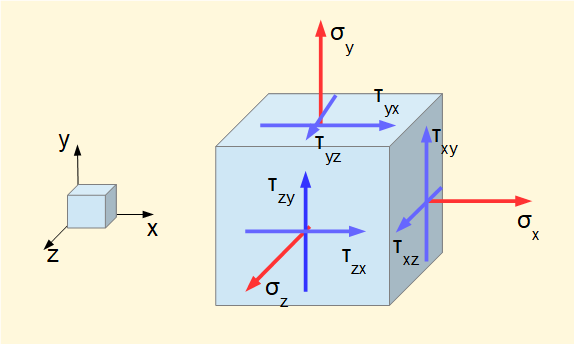
Normal stress σ and shear stress τ are positive when acting in the positive direction of the references axes. Thus all stresses in this diagram are positive.
For equilibrium τxy= τyx τyz= τzy τzx= τxz
Note the convention for designating shear stresses – the first subscript is the co-ordinate normal to the face; the second subscript is the axis parallel to the face.
Corresponding stresses exist on the three hidden faces of the element. Directions of these stresses are such as to maintain static equilibrium of the element.
For some situations a two-dimensional (biaxial or plane) stress analysis suffices where we consider stresses acting on planes perpendicular to the x and y axes.
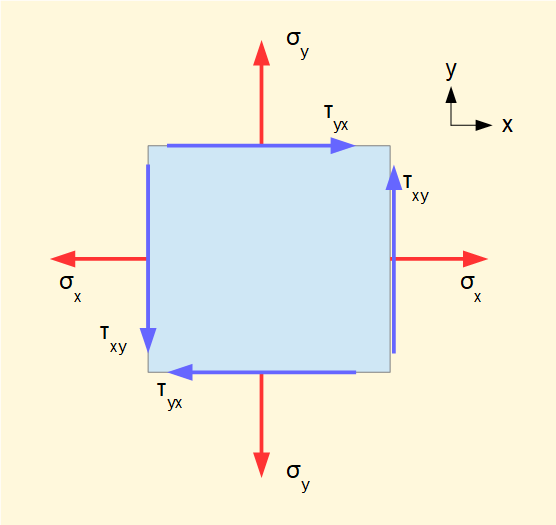
Directions of σ shown are positive and represent tension; reverse directions represent compression.
Directions of τ are designated clockwise (cw) or counter-clockwise (ccw). In the diagram τyx is clockwise (cw) and τxy is counter-clockwise (ccw).
Mohr's circle of stress
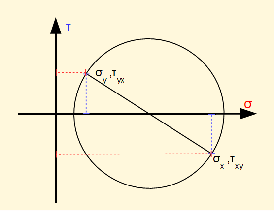
We will now show a graphical method of determining normal and shear stresses based on known values of σx σy τxy τyx where the stress element is oriented at any angle θ to the xy axes using a diagram known as Mohr's circle of stress.
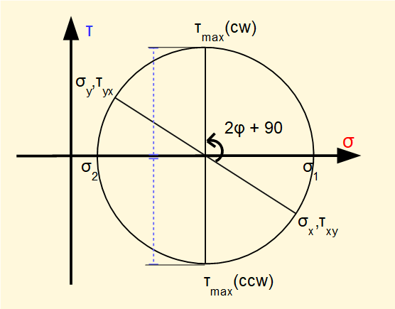
To construct Mohr's circle set out orthogonal axes of σ and τ. Mark off the known values of σx,τxy and σy,τyx. The line joining these points forms the diameter of the circle. The angular orientation of this diameter represents the reference axes xy.
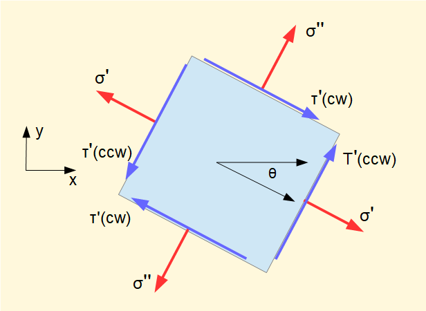
Now consider stresses σ/ , σ//, τ/(cw) and τ/(ccw) on planes rotated clockwise by angle θ.
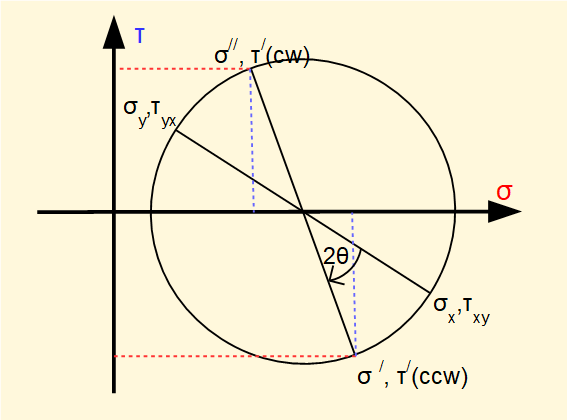
These stresses are resolved on Mohr's circle by rotating the base diameter through angle 2θ and projecting from the circumference on to the σ and τ axes. Note shear stresses are of equal magnitude on all four faces.
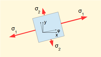
Now consider a specific rotation of the planes through angle φ anti-clockwise relative to the reference xy axes.

The circle diameter rotates through angle 2φ anti-clockwise, being the angle that brings the base diameter coincident with the σ axis. Hence there are no shear stresses on these planes. We call these normal stresses the principal stresses, designated σ1 and σ2 shown on the diagram below.
The principal stresses act on the principal planes which are 90° apart (180° on the Mohr circle).
It is clear from the diagram that the principal stresses σ1 and σ2 are respectively the maximum and minimum normal stresses.
It is also clear from Mohr's circle below that the maximum shear stress occurs on planes oriented 45° (90° on the circle) from the principal planes. It is easily shown that normal stresses are equal on the planes of maximum shear stress and have the value (σ1 + σ2}/2 where σ1 and σ2 are the principal stresses.
Equations used to derive Mohr's circle can be found in standard text books and provide a means of calculating normal and shear stresses on the faces of an orientated element.
Strain
Materials subject to normal stress σ experience deformation which in general terms we call strain.
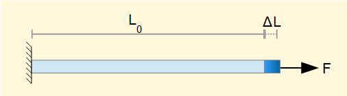
The diagram above shows a bar of material length L0, with applied axial force F. The elongation of the bar is ΔL and the strain ε is defined as:
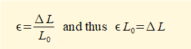
Note that this definition of strain has no dimensions. The diagram shows the tensile strain resulting from tensile stress in the bar. A compressive force produces compressive strain.
Sometimes the term total strain is used for ΔL, i.e. the actual elongation or compression of the material. The units of ΔL are length units.
When material such as a round bar in the diagram below is subject to longitudinal tensile strain there is a corresponding contraction in the lateral direction. Conversely there is lateral expansion in a bar subject to compressive strain. The respective elongations and contractions are shown where εx is the longitudinal strain and εy the lateral strain.
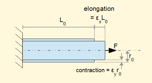
Provided the material under load remains in the linear-elastic range for stress and strain (see below) the ratio between εy and εx is effectively constant. This constant is designated ν (Greek Nu) and known as Poisson's ratio.
For most engineering materials the value of ν is approximately 0.3
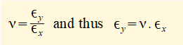
We have considered strain resulting from normal stresses σ. Strain arising from shear stress τ is defined in the diagram below.
The biaxial stress condition shows a rectangular block of material deformed under shear stress τ into the form of a parallelogram. The angle γ defines the shear strain. As with ε, shear strain has no dimensions and is measured in radians.
Relation between stress and strain
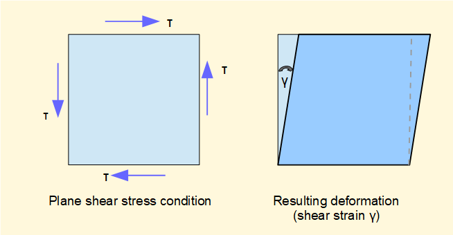
The diagram below illustrates the relation between stress and strain in the linear-elastic range for a material.
Stress-strain diagrams such as this are generally obtained from tensile load tests using a test piece in the form of a round bar. As the load on the test piece increases the stress increases and the resulting strain is measured.
The diagram shows a linear relationship between stress and strain up to a point called the proportional limit, sometimes called the elastic limit. In this region the material is said to be elastic, meaning that when the load is removed it regains its original dimensions without deformation.
In the linear-elastic region the relationship between stress and strain is expressed as:
σ = E. ε where the constant E is called Young's modulus or the modulus of elasticity.
Note that E has the same units (Pa) as stress. E is a measure of the stiffness of a material, the greater the value of E the stiffer the material.
For most engineering materials the strain in the linear-elastic region is very small, typically up to 0.001. Behaviour beyond the elastic limit is outside the scope of this tutorial but in broad terms materials reach a yield point beyond which increasing stress produces permanent deformation and eventually fracture. There are significant differences in behaviour between ductile and brittle materials.
Values of E vary considerably for different materials. Typical values are:
carbon steel E = 207 GPa
brass E = 106 GPa
cast iron E = 100 GPa
aluminium alloy E = 70 GPa
Material subjected to pure shear stress also exhibits linear-elastic behaviour. In this case the relation is:
τ = G.γ where the constant G is called the modulus of rigidity or shear modulus.
Again, G has the same units (Pa) as stress. Values of G are generally about 1/3 those of E.
To complete this overview of the basic concepts of stress and strain we will look again at the condition of triaxial stress (see above) where the element is aligned on the axes of the principal stresses and thus shear stresses are zero on all faces of the element. The strains associated with the principal stresses are called principal strains.
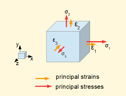
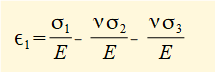
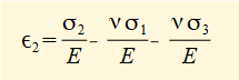
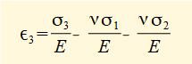
The diagram above shows principal strains produced on each axis for an arbitrary set of tensile principal stresses where σ1 > σ2 > σ3. Note that tensile principal stress can be accompanied by compressive strain on the same plane. The following general relations between principal stresses and principal strains are derived from the definition of Poisson's ratio ν.
Next: Beams - Terminology and sign conventions
I welcome feedback at: