In the introductory tutorial in this series we considered a free vibrating translational spring and mass system with one degree of freedom and no external force applied as shown in Figure 1 below. Mass m connected to a spring with spring constant k with static equilibrium position x = 0 is free to move on a horizontal frictionless plane. The diagram shows the force Fs exerted by the spring on mass m, (i) in extension and (ii) in compression.
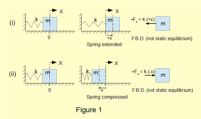
The free body diagrams show Fs = -k.x at all positions of x in the oscillating cycle. This force must equal the acceleration a of mass m by Newton's Law.
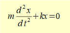
This equation is an expression of simple harmonic motion in that acceleration is always directed towards the equilibrium point and is directly proportional to the distance from that point.
Solution to the equation of motion
We now find a function x(t) that is a general solution to this equation. If you are not familiar with solving second-order homogeneous linear differential equations using the characteristic equation method study the maths tutorial.

Note that k has dimensions ML / T2L (force / displacement). Thus ω2 and ω = √(k/m) have dimensions respectively 1/T2 and 1/T.
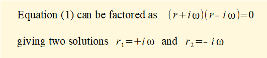
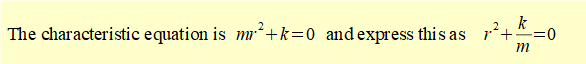
From the maths tutorial we see that two complex conjugate roots of the characteristic equation expressed as:
r1 =( α + iβ) and r2 = (α - iβ) give the following general solution for x = f(t):
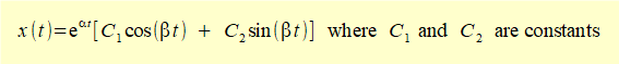
In the case above r1 = +i.ω and r2 = -i.ω Thus α = 0 and β = ω giving the general solution for the equation of motion as:
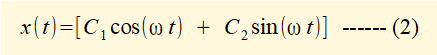
It is conventional to replace constants C1 and C2 with A and B giving:
x(t) = [Acos(ωt) + Bsin(ωt)] ---------- (3)
We now find a particular solution for equation (3) using the following initial conditions at time t = 0 :
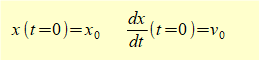
Meaning at time t = 0 the extension of the spring is x0 and the mass has initial velocity v0.
Inserting initial condition x0 into equation (3) at time t = 0 gives:
x0 = Acos(ωt) + Bsin(ωt) = (A).(1) + (B).(0) = A thus A = x0

v0 = -ωA.sin(ωt) + ωB.cos(ωt) = -ωA.(0) + ωB.(1) thus B = (v0 / ω)
x(t) can now be expressed in terms of initial conditions x0 and v0 as;
x(t) = x0cos(ωt) + (v0 / ω) sin(ωt) ------- (4)
It is convenient to express the equation of motion in terms only of cos(ωt) using the following identity:
Acos(ωt) + Bsin(ωt) = Rcos(ωt - φ) where R = √(A2 +B2) and φ = tan-1 B /A
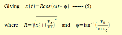
R is the maximum absolute value of x(t) called the amplitude of the oscillation.
ω represents the angular frequency of the oscillation in radians/sec. This is also the natural frequency of the free vibrating system denoted by ωn.
Note that:
- ωn / 2π is the natural frequency measured in Hertz (Hz).
- The period T (seconds)of one cycle is the reciprocal of the frequency = 2π / ωn.
Example
Figure 2 below plots displacement x(t) = R1.cos(ωt - φ) against time t for a spring and mass system with the following parameters:
- mass m = 1 kg
- spring constant k = 10 N/m
- initial displacement x0 = 0.1 m
- initial velocity v0 = 1 m/s
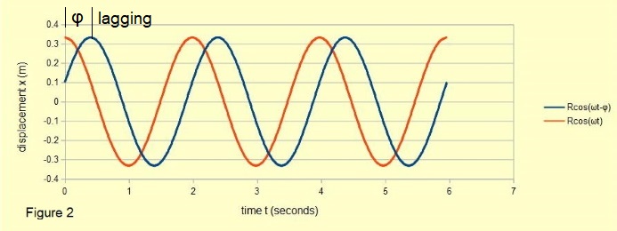
For this system with the above initial conditions:
- natural frequency ωn = √(k/m) = √(10) rad/sec equivalent to (ωn/2π) = 0.503 Hz.
- period T = (2π/ωn ) = 2π/√(10) = 1.99 s
- amplitude R1 = √([x02 + (v0/ωn)2] = √([0.12 + (1/√((10))2] = 0.332 m
- phase angle φ = tan-1(v0/ωnx0) = tan-13.162 = 72.45°
Phase angle is measured relative to motion of the same spring and mass system where the initial velocity is zero.
Such a condition is shown in Figure 2 by the plot for x(t) = R2cos(ωt) with initial conditions:
- x0 = 0.1 m
- v0 = 0
giving R2 = 0.1 m
Note that natural frequencies of both motions are identical since ωn depends only on k and m. The phase angle φ between the two oscillations in this example = 72.5° with R1cos(ωt - φ) lagging R2cos(ωt).Next: Free vibrations with damping
I welcome feedback at: