In the introductory tutorial in this series we considered a free vibrating translational spring and mass system with one degree of freedom with viscous damping as shown in Figure 1 below. Mass m connected to a spring with spring constant k is free to move on a horizontal frictionless plane from the static equilibrium position x = 0.
A dashpot provides a damping force F = -c.v where v is velocity of mass m and c the damping coefficient.
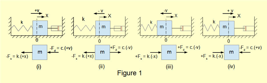
The diagram shows free body diagrams of forces on mass m at four phases of the oscillating cycle from which we obtained the following equation of motion for this system:
We now find a function x(t) that is the general solution to this equation. If you are not familiar with solving second-order homogeneous linear differential equations using the characteristic equation method study the maths tutorial.
In the previous tutorial we found that k/m = ωn2 where ωn is the natural frequency of the undamped system.
Roots r1 and r2 of this equation from the quadratic formula are:
We now manipulate this expression as follows to provide a dimensionless factor ζ (zeta) called the damping ratio.
(Dimensions of the parameters of ζ are: c = M/T, ωn = 1/T, m = M)
From the maths tutorial we know the general solution to the equation of motion using roots r1 and r2 of the characteristic equation is:

We now examine the general forms of this solution where:
- ζ > 1
- ζ = 1
- ζ < 1
Solutions where ζ > 1

If ζ > 1:
- √(ζ 2 - 1) is positive, meaning that solutions are real numbers and can be obtained directly from equation (3).
- √(ζ 2 - 1) < ζ thus [- ζ ± √(ζ 2 - 1)] must be negative. Since ωn is always positive, it follows that both r1 and r2 must be negative. Therefore the motion must have a decreasing exponential characteristic.
Example
The following example illustrates a damped spring, mass and dashpot system where ζ > 1. Initial conditions at time t0 are:
- x(t) = x0
- dx(t)/dt = v0
Derive expressions for constants C1 and C2 in equation (3) as follows:

At time t = 0:
- x0 = C1 + C2
- v0 = dx/dt = a.C1 + b.C2 (e0 = 1)
Solving for C1 and C2 gives:

Figure 2 below shows a plot of x(t) against time t for a damped free vibrating system with the following parameters:
- m = 1.0 kg
- k = 10 N/m
- c = 12 Ns/m
- x0 = 0.1 m
- v0 = 1.0 m/s
- ωn = √(k/m) = √(10) rad/sec
- ζ = c/2.ωn.m = 12/2.√(10) = 1.90
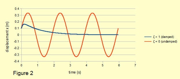
The motion characterised by ζ > 1 which decreases exponentially with time to the limit x(t) = 0 is defined as aperiodic, also described as heavily damped. For comparison undamped motion of the equivalent free vibrating system (ζ = 0) derived in the previous tutorial is also plotted.
Solutions where ζ = 1
If ζ = 1:
it follows that ωn[- ζ ± √(ζ 2 - 1)] = - ωn
From the maths tutorial we know the general solution to this equation is:

To find constants C1 and C2 in equation (4) apply initial conditions x0 and v0 at time t = 0

Figure 3 below shows a plot for x(t) against time t for the system with ζ = 1 using the values for m, k and initial conditions for displacement (x0) and velocity (v0) from the previous example.
In this case the damping coefficient c = 2.ωn.m.ζ = 6.32 Ns/m
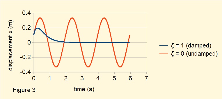
The motion characterised by ζ = 1 is also aperiodic and has the shortest time for decay to the limit where x(t) = 0 (compare with Figure 2 for ζ > 1). It is called the critically damped condition.
Solutions where ζ < 1
If ζ < 1:
it follows that (ζ 2 - 1) is negative; thus r1 and r2 are complex numbers.
From the maths tutorial we know the roots* are:
r1 = α + i β and r2 = α - i β where α = -ωn.ζ and β = ωn√(1 - ζ 2)
*using the transformation √(ζ 2 - 1) = √[(-1)(1 - ζ 2)] = i.√(1 - ζ 2 )
To find constants C1 and C2 in equation (5) use initial conditions x0 and v0 at time t = 0
For t = 0 equation (5) reduces to: x0 = C1

which for v0 = dx/dt at time t = 0 gives:


Figure 4 below shows a plot of x(t) against time t for the system with ζ < 1 using the values for m, k and initial conditions x0 and v0 from the previous examples. In this case the damping ratio ζ = 0.1 and the damping coefficient c = 0.63 Ns/m.
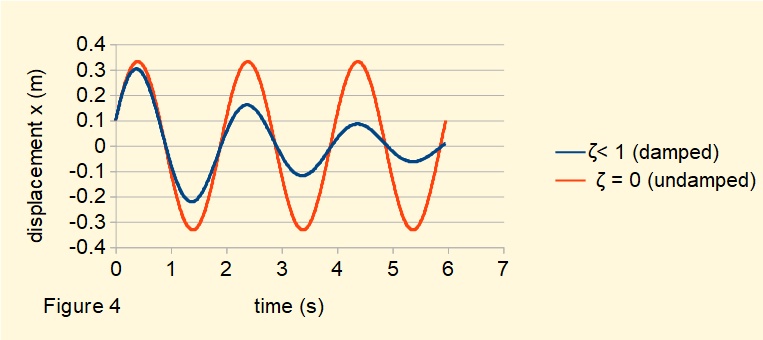
When ζ < 1 damping produces a decaying oscillatory motion, often described as light damping. As it is the most important mode of vibration in engineering applications we examine the characteristics in more detail.
Characteristics of light damping (ζ < 1)
Consider the general solution to the equation of motion for damped free vibration when the damping ratio ζ < 1 derived above:

where α = -ωn.ζ and β = ωn√(1 - ζ 2)
From the maths tutorial we know this equation can be expressed as:

Substituting for α and β gives:

where A = √((eαt.C1)2 + (eαt.C2)2) and φ = tan-1(eαt.C2) / eαt.C1
Equation (6) can be interpreted as damped oscillatory motion in two parts.
1. cos[(ωn(√1 - ζ 2 ).t - φ]
This expression represents harmonic motion at frequency ωn√(1 - ζ 2 ). We call this the damped natural frequency ωd which differs from the natural frequency of the free vibrating system ωn by the factor √(1 - ζ 2 ).
In most practical applications ζ << 1 and ωd ≈ ωn . In the example above ζ = 0.1 and √(1 - ζ 2 ) = 0.995. This deviation is impossible to detect on the plot in Figure 4.
2. A.e-ζ.ωn.t
This expression represents exponential decay of the damped motion designate xexp(t).
xexp(t) = A.e-ζ.ωn.t Thus when t = 0 xexp(0) = A
It is conventional to designate A = X0 and express the exponential decay as xexp(t) = X0.e-ζ.ωn.t
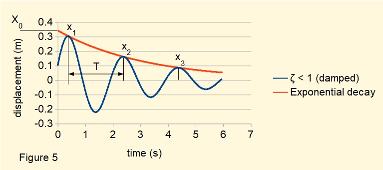
Figure 5 below plots the damped natural frequency from Figure 4 with the exponential decay computed from the expression X0.e-ζ.ωn.t.
Method of estimating damping ratio ζ
We obtained the plot in Figure 5 by assigning a known value to the damping ratio ζ. It is useful to have an practical method of estimating the value of ζ by measuring displacement of the system mass against time. The following method involves measuring displacement at successive peaks in the decaying motion.
From Figure 5 the period of each cycle of the decaying harmonic motion is T. The ratio of the peak displacements between n cycles can be expressed as;
where x(t) is the first measured peak and x(t + nT) is the peak after n successive cycles.

Constant A and the cosine* terms cancel giving:
*cosine terms in denominator are multiples of term in numerator at intervals of 2π
Typically ζ << 1 thus √(1 - ζ 2) ≈ 1 giving:
Example
Estimate the value of ζ from the plot in Figure 5
Use peaks x1 = 0.30 m and x3 = 0.08 m for which n = 2.
This is a very good approximation, ζ = 0.1 being the value assigned to the system represented by the plot in Figure 5.
This has been meaty tutorial but if you take the maths slowly step by step to their conclusions interpreting the results is rewarding.
Next: Forced vibrations without damping
I welcome feedback at: