Mechanical vibrations - introduction and overview
Introduction
I have chosen mechanical vibrations as a topic for a series of tutorials largely because I did not give the subject sufficient attention as engineering student many years ago. I recall the maths being somewhat daunting so in these tutorials I present the maths step by step supported by a maths tutorial for methods of solving second order ordinary differential equations.
This first series of tutorials considers single degree of freedom systems with translational motion* and includes analysis of:
* As opposed to angular motion.
- free vibrations
- free vibrations with damping
- forced vibrations without damping
- forced vibrations with damping
In this introductory tutorial we examine spring and mass models for each of the above systems, with viscous damping where appropriate, and establish the differential equations of motion where displacement x and time t are respectively the dependent and independent variables. In the subsequent tutorials we solve these equations and illustrate physical responses.
I have taken particular care to illustrate the signs of parameters in free body diagrams when deriving these equations. To my mind most text books do not give this aspect sufficient attention.
Free vibrations
The spring and mass model for a free vibrating system with one degree of freedom is shown in Figure 1 below. Vector quantities directed along the x axis to the right are positive and to the left are negative.
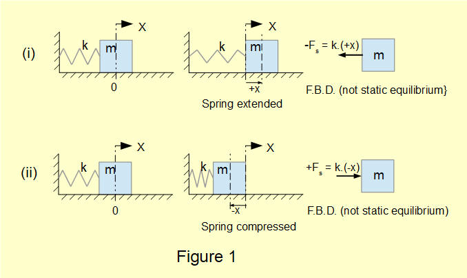
In this system mass m is attached to a spring and is free to move on a frictionless horizontal plane on axis X. In this idealised condition there is no damping to remove energy from the system. The diagrams on the left show the spring and mass at x = 0 with no force exerted on the mass by the spring which is in its equilibrium state. According to Hooke's law the extended or compressed spring exerts a force Fs on the mass directly proportional to the displacement x and opposed to the displacement from the spring equilibrium position (in this case x = 0) . This constant of proportionality is called the spring constant, denoted by k with units N/m.
With reference to the X axis in Figure 1 we can express the spring force acting on mass m as follows : (i) where x > 0 - Fs = k.(+x) (ii) where x < 0 +Fs = k.(-x) We can generalise both (i) and (ii) as Fs = - (k.x)
Free body diagrams (FBDs) for conditions (i) and (ii) do not show a condition of static equilibrium but are a snapshot of the mass in motion*. Thus Fs is the only external force acting on the mass. From Newton's second law it follows that Fs = m.a (where a is the acceleration of mass m) and thus m.a = -(k.x)
* A "pseudo" inertial force in accordance with D'Alembert's principle is not inserted because the FBD does not show a static equilibrium condition.
We conclude from this equation that the motion of the spring and mass system is simple harmonic motion (SHM) as it fulfils the definition of SHM, namely that a body moves with SHM if its acceleration is directly proportional to its displacement from a fixed point and is always directed towards that point. In this case the fixed point is the equilibrium position of the spring at x = 0.
The solution to this equation of motion and its interpretation is the subject of a separate tutorial.
Free vibrations with damping
To represent damping we add viscous friction to the free vibration model of Figure 1 in the form of a "dashpot" shown in Figure 2 below. The dashpot is a piston and cylinder filled with a viscous liquid. Liquid flowing from one side of the moving piston to the other provides a controlled amount of resistance to movement. This damping force Fd is directly proportional to v the velocity of the piston. This constant of proportionality c is called the damping coefficient with units Ns/m.
Coulomb friction, which is not proportional to velocity, can also contribute to damping but is not included in this model.
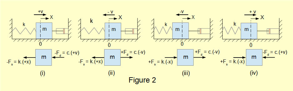
The figure shows the damping force Fd in a spring and mass vibrating system for positive and negative velocities v. It is instructive to consider FBDs* showing spring force Fs and damping force Fd for four dynamic conditions:
* Note again that these FBDs do not illustrate static equilibrium conditions
- (i) spring extension (x is +ve) and v is +ve,
- (ii) spring extension (x is +ve) and v is -ve
- (iii) spring compression (x is -ve) and v is-ve
- (iv) spring compression (x is -ve) and v is +ve.
It can be seen that for each of the above conditions Fd = - (c.v). It also follows for each condition that the total external force on mass m FTotal = - (k.x) - (c.v)
Again by Newton's second law FTotal = m.a = - (k.x) - (c.v)
The solution to this equation of motion and its interpretation is the subject of a separate tutorial.
Forced free vibrations
We now consider the effect of applying an external force to a spring and mass system, in this first case without damping. The applied force is called a forcing function and we consider a harmonic function Ff = F0cos(ωt)* where ω in radians/sec is the angular frequency of the periodic function and F0 is the amplitude in units of force.
* choosing cos(ωt) as the forcing function determines that at time t = 0 Ff = F0 since cos(ωt) = 1. It is equally valid to choose sin(ω t) as the function in which case at t = 0 Ff = 0

Figure 3 above shows the "dynamic" FBD for the system with Ff applied when the spring is extended and the velocity of the mass is +ve. The total external force on mass m FTotal = + F0cos(ωt) - (k.x). Again by Newton's second law FTotal = m.a = + F0cos(ωt) - (k.x).
which gives the equation of motion for a free vibrating system with an applied harmonic forcing function as:

The solution to this equation of motion and its interpretation is the subject of a separate tutorial.
Forced free vibrations with damping
We now add damping to the free vibrating system with a harmonic forcing function considered in the previous section.
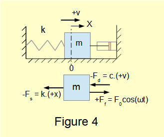
Figure 4 above shows the corresponding "dynamic" FBD with the viscous damping force (- Fd) = c.(+v) where c is the damping constant. It follows that the total external force FTotal acting on mass m is: FTotal = m.a = + F0cos(ωt) - (c.v) - (k.x)
which gives the equation of motion for a free vibrating system with an applied harmonic forcing function as:

The solution to this equation of motion and its interpretation is the subject of a separate tutorial.
Summary
We now have four differential equations of motion which are the basis for the next four tutorials in this series.
These equations which have displacement x as the dependent variable and time t as the independent variable are second order ordinary linear differential equations. The first two are homogeneous equations because the RHS equals 0. The latter two where the RHS is a function of the independent variable are non-homgeneous equations. The maths tutorial for this series provides a summary of methods for solving both types of equation. An understanding of these methods is necessary for the remainder of the tutorials in this series.
I welcome feedback at: