In the introductory tutorial in this series we considered a harmonic forcing function F0cos(ωt) applied to a translational spring and mass system with one degree of freedom having mass m, spring constant k and a dashpot providing viscous damping with damping constant c shown in Figure 1 below with the spring extended by distance x.
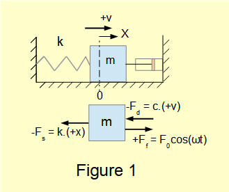
From the dynamic* free body diagram we obtained the following equation of motion in terms of displacement x and time t:
*sum of forces produces acceleration of mass m, not static equilibrium
We now find a function x(t) that is a general solution to this equation.
the maths tutorial in this series provides an outline of solutions to homogeneous and non-homogeneous second-order ordinary differential equations
Recall that the general solution to a second-order non-homogeneous ordinary linear differential equation is:
+
For forced vibrations with damping the first part of the solution is the general solution to the homogeneous differential equation of motion for damped free vibrations derived in a previous tutorial as follows:
where C1 and C2 are constants, ωn is the natural frequency of the spring and mass system
and ζ = c/2ωn.m is the damping ratio
We also showed that all particular solutions of equation (2) (where ζ > 1, ζ = 1 and ζ < 1) have the characteristic that x(t) → 0 as time increases and can thus be considered a transient condition for forced vibrations with damping.
In this tutorial we are interested in the steady state condition which is defined by the particular solution to equation (1) as this has much greater practical significance. Hence we will only consider the particular solution.
Find the particular solution to equation (1)
We know that the particular solution to equation (1) will be a harmonic function in ωt where ω is the angular frequency of the forcing function and will have the form:
xp = A.cos(ωt) + B.sin(ωt) where A and B are unknown values of displacement x(t).
This expression can also be stated in the form:
xp = X.cos(ωt - φ) ------ (3)
where X is an unknown value of x(t) and φ is an unknown value of phase angle.
We now proceed to solve equation (3) for unknowns X and φ.
Firstly, substitute xp, dxp/dt and d2xp/dt2 derived from equation (3) into equation (1) to give:

Now divide by k to give:
*see a previous tutorial for the derivation of damping ratio ζ
We now create two equations from equation (4) to provide solutions for the two unknowns, X and φ using the following trig identities:
(i) cos(ωt - φ) = cos(ωt).cos(φ) + sin(ωt).sin(φ)
(ii) sin(ωt - φ) = sin(ωt).cos(φ) - cos(ωt).sin(φ)
X.cos(ωt).[A.cos(φ) + B.sin(φ)] + X.sin(ωt).[A.sin(φ) - B.cos(φ)] = (F0/k).cos(ωt) ------- (5)
By equivalence of coefficients in equation (5) for cos(ωt) and sin(ωt) terms gives the following:
(i) X.[A.cos(φ) + B.sin(φ)] = (F0/k) ---- (6)
(ii) X.[A.sin(φ) - B.cos(φ)] = 0 ---- (7)
Solving simultaneous equations (6) and (7) gives the following solutions for X and φ :
Substituting back for A and B gives:
which completes the solution for equation xp = X.cos(ωt - φ) representing the steady state condition of a damped forced vibration with forcing function F0cos(ωt). where:
X is the amplitude of displacement and φ the phase angle of displacement relative to the harmonic forcing function.
Characteristics of steady state response
Note: for practical application we express the equation for steady state response as:
x(t) = X.cos(ωt - φ)
In the analysis below we use the following important parameters:
- frequency ratio = ω/ωn which is the ratio of the frequency of the harmonic forcing function and the natural frequency of the spring and mass system.
- damping ratio ζ = c/2ωn.m which is a dimensionless factor expressing the degree of damping in the system.
- static amplitude δ = (F0/k) which expresses the static displacement of mass m subject to force F0 in a spring and mass system with spring constant k.
- amplification factor (X/δ) which expresses the amplification effected by the forcing function relative to the static displacement.
Examples
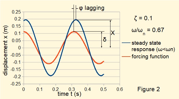
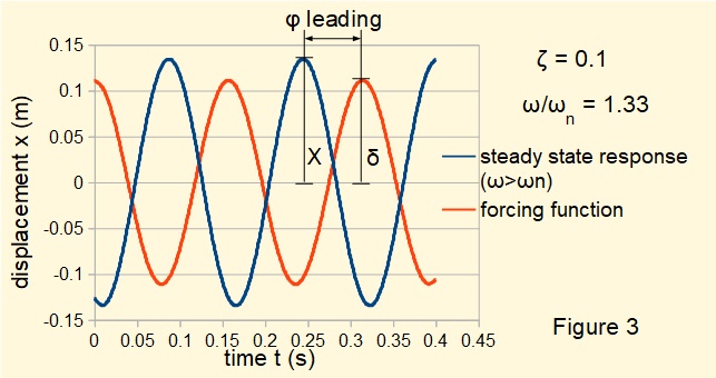
The following two examples plot steady state response of a damped spring and mass system to a harmonic forcing function F0cos(ωt). Damping ratio of the system ζ = 0.1.
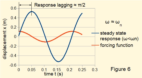
Figures 2 below plots the steady state response for a system where frequency ratio ω/ωn < 1 . The amplification factor (X/δ) ≅ 1.75.. Response lags the forcing function.
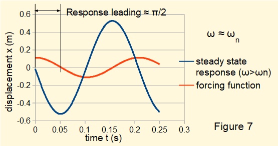
Figures 3 below plots the steady state response for a system where frequency ratio ω/ωn > 1 . The amplification factor (X/δ) ≅ 1.21. Response leads the forcing function.
General characteristics of steady state response
General characteristics of steady state response over a wide range of system parameters are illustrated in Figures 4 and 5 below.
Figure 4 below plots amplification factor (X/δ) against frequency ratio ω/ωn for three values of damping ratio ζ.
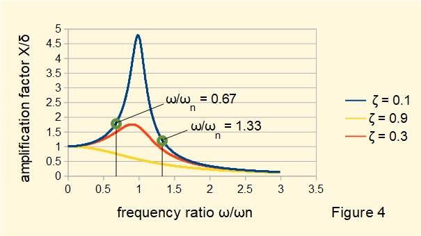
Note the following from Figure 4:
- The amplification factor peaks at a frequency ratio dependent on ζ. The peak amplification factor occurs closer to frequency ratio = 1 as ζ tends to zero, which is the resonant condition for undamped systems derived in the previous tutorial.
- For all values of ζ the amplification factor tends to zero as frequency ratio increases beyond the peak value.
- The frequency ratios used to compute the plots in Figures 2 and 3 above are indicated on the plot line for ζ = 0.1.
Figure 5 below shows the variation of phase angle φ (units in radians) with frequency ratio for three values of damping ratio ζ.
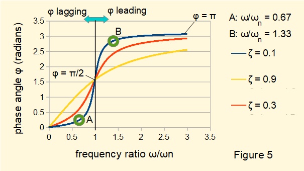
Note the following from Figure 5:
- At frequency ratios < 1 displacement x(t) lags the forcing function. Phase angles increase from zero to π/2 as the frequency ratio increases to 1.
- At frequency ratios > 1 displacement x(t) leads the forcing function. Phase angles increase from π/2 to π as the frequency ratio increases.
- The frequency ratios used to compute the plots in Figures 2 and 3 above are indicated on the plot line for ζ = 0.1.
- At frequency ratio = 1 there is an unstable condition where the phase angle transitions from π/2 lagging to π/2 leading.
Figures 6 and 7 below illustrate the transformation of phase angle from lagging to leading where ω/ωn is respectively fractionally less than and fractionally grater than 1.
This tutorial concludes the series on mechanical vibrations at present.
Return to: Mechanical vibrations - content
I welcome feedback at: