Forced vibrations without damping

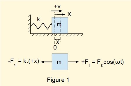
In the introductory tutorial in this series we considered a harmonic forcing function F₀cos(ωt) applied to a translational spring and mass system oscillating on a frictionless horizontal plane with one degree of freedom. This system with mass m and spring constant k is shown in Figure 1 below with the spring extended by distance x

It should be understood that a completely undamped spring and mass oscillating system does not exist. Friction forces will in time dissipate the initial transient response after which the forcing function produces a steady state response. However, analysing the response to a forcing function of a system with no explicit damping term has merit in that it introduces important concepts, in particular the property of resonance.

From the dynamic* free body diagram shown in Figure 1 we obtained the following equation of motion in terms of displacement x and time t

*sum of forces produces acceleration of mass m, not static equilibrium

We now find a function x(t) that is a general solution to this equation. If you are not familiar with solving second-order non-homogeneous ordinary linear differential equations using the method of undetermined coefficients refer to the maths tutorial.

From the maths tutorial recall that the general solution to a second-order non-homogeneous ordinary linear differential equation is:

+

Step 1

Thus the first step is to find the general solution x_h(t) to the complementary homogeneous equation:

From a previous tutorial we know the general solution to this equation is:

Step 2

We now propose a particular solution x_p(t) to equation (1) of the form:

x_p(t) = [A.cos(ωt) + B.sin(ωt)]

where A and B are undetermined coefficients and ω is the frequency of the harmonic forcing function.

Step 3

The general solution to equation (1) is    x_h(t) +x_p(t)   giving:

Equation (3) is a valid solution for all values of ω except ω = ω_n which gives a duplicate solution containing the function cos(ω_nt). The proposed particular solution for this condition takes the form:

x_p(t) = [A.t.cos(ω_nt) + B.t.sin(ω_nt)]   which we develop later.

Meanwhile continuing with a particular solution to equation (1) for ω ≠ ω_n we find constants C₁ and C₂ for initial conditions x₀ and v₀ at time t = 0 where v₀ = dx(t)/dt.

Thus from equation (3) the particular solution for equation (1) for initial conditions x₀ and v₀ is:

Resulting motion

We now explore characteristics of the forced vibratory motion defined by equation (4).

To simplify the analysis:

Recall that   k = m.ω_n²

The first term in equation (5) with cos(ω_nt) derived from the general solution expresses the transient response attributable to the free vibration of the system. In practice this response dissipates because of friction.

The second term in equation (5) with cos(ωt) derived from the particular solution expresses the steady state response.

Steady state response

Using the second term in equation (5) for steady state response giving:

we consider steady state response for three conditions:

• ω > ω_n


• ω < ω_n


• ω = ω_n

where ω is the frequency of the harmonic forcing function and ω_n is the natural frequency of the free vibrating system.

We introduce a useful parameter of the forcing function called the static amplitude δ = (F₀ / k) expressing the static displacement of mass m under force F₀.

If X is the amplitude of the harmonic steady state response, the factor X/δ called the amplification factor is a measure of the amplification effected by the forcing function.

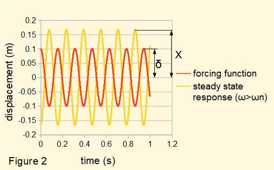
1. Consider   ω > ω_n

Figure 2 below plots the steady state response of the system when the frequency of the forcing function ω > ω_n. Note the response is out of phase with the forcing function by 180°.

In this example frequency ratio ω/ω_n = 1.26. Amplification factor (X/δ) ≈ 1.6.

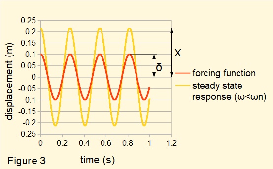
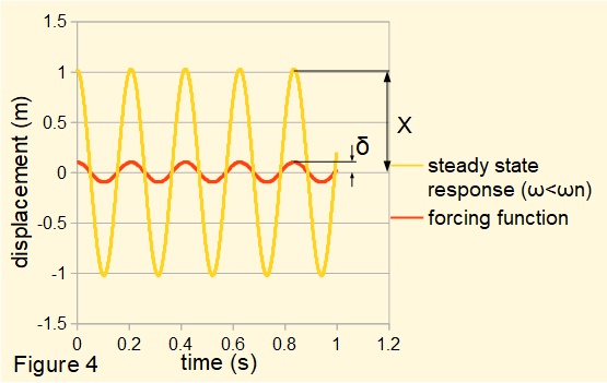
2. Consider   ω < ω_n

Figure 3 below plots the steady state response of the system when the frequency of the forcing function ω < ω_n. Note the response is in phase with the forcing function.

In this example frequency ratio ω/ω_n = 0.73. Amplification factor X/δ ≈ 2.2.

The general characteristics illustrated in Figures 2 and 3 can be deduced as follows.

Consider the term in equation (5) representing steady state response:

with respect to forcing function F₀cos(ωt):

(a)   If ω > ω_n the coefficient X is negative and thus out of phase with the forcing function by 180°.

(b)   If ω < ω_n the coefficient X is positive and thus in phase with the forcing function.

(c)   The smaller the difference between ω and ω_n the greater the amplification factor X/δ.

Figure 4 below illustrates characteristic (c). Amplification factor X/δ ≈ 10 when frequency ratio ω/ω_n = 0.95

3. Consider   ω = ω_n

Figure 5 below shows the relationship between the frequency ratio ω/ω_n and the absolute value of amplification factor X/δ.

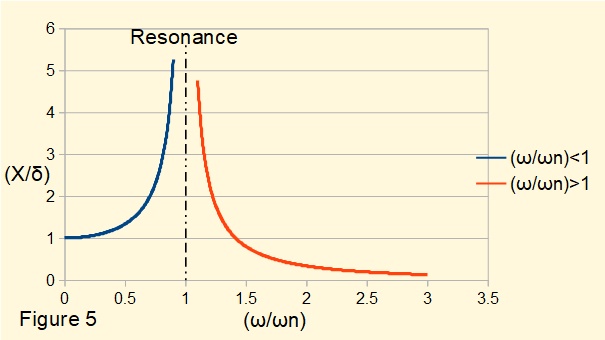
Note the different characteristics as ω approaches ω_n for ω < ω_n and ω > ω_n.

This condition when ω is very close to or equals ω_n is known as resonance where the theoretical amplification factor tends to infinity. In practice physical constraints limit the amplitude of vibration.

Combined transient and steady state response

Figures 2 to 5 illustrate the steady state condition of a free vibrating system subjected to a harmonic forcing function after transient effects are eliminated by the small amount of damping inherent in the system. We now consider the response including the transient term in cos(ω_nt) from equation (5).

Figures 6 and 7 below are plots for equation (7) with parameters ω = 40 rad/s and ω_n = 30 rad/s (frequency ratio = 0.75) giving the equation:

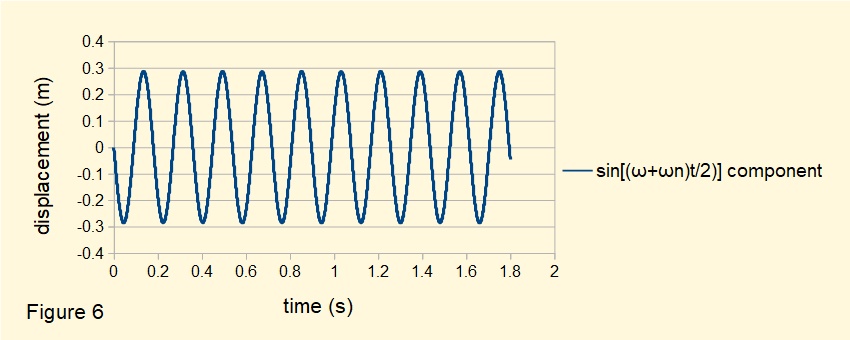
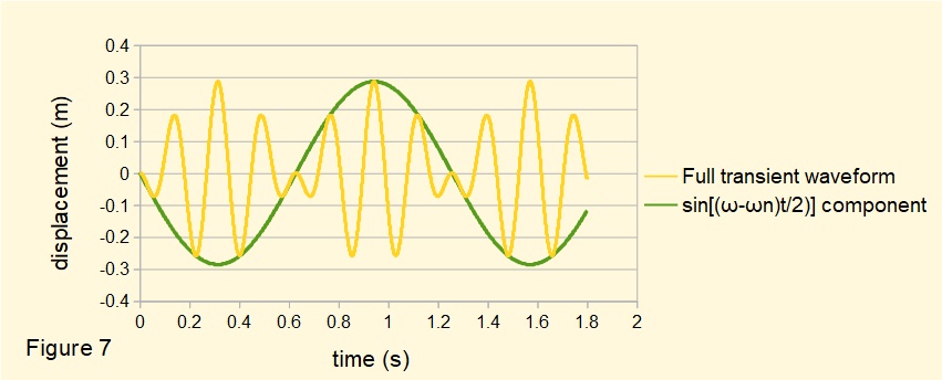
Figure 6 plots the waveform for the sin[(ω + ω_n)/2] component of equation 8.

Figure 7 plots the full waveform of equation 8 with the waveform for the sin[(ω - ω_n)/2] component superimposed.

These waveforms illustrate the phenomenon of beating where the amplitude varies periodically in a regular pattern. In this example the frequency of the resultant waveform is a function of sin(35t) and the envelope of the beat is a function of sin(5t). Beating can often be detected in sound waves generated by vibration.

General solution to equation for condition ω = ω_n

For the final part of this tutorial we develop a general solution to the equation:

for the condition where ω = ω_n.

Recall that the general solution to non-homogeneous equation (1) comprises two parts. The first part is the general solution to the complementary homogeneous equation which in a previous tutorial was found to be:

The second part of the general solution is a particular solution to the non-homogeneous equation.

Recall from above that the particular solution x_p(t) = [A.cos(ωt) + B.sin(ωt)] for conditions where
ω > ω_n and ω < ω_n was not valid for the condition ω = ω_n.

The proposed particular solution for the condition ω = ω_n takes the form*:

x_p(t) = [A.t.cos(ω_nt) + B.t.sin(ω_nt)] --------- (9)

* by the reduction of order method referred to the maths tutorial

To find undetermined coefficients A and B in equation (11) let initial condition t = 0

gives:   2m.ω_nB - 0 = F₀

Thus:   B = F₀/2m.ω_n

Substitute in equation (11) for B

Gives   F₀.cos(ω_nt) - 2m.ω_nA = F₀.cos(ω_nt)

Thus   A = 0

Substituting for A and B in equation (9) gives the particular solution for condition ω = ω_n as:

Thus the general solution to equation (1) for condition ω = ω_n is:

From equation (12) find constants C₁ and C₂ for initial conditions x₀ and v₀ at time t = 0
where v₀ = dx(t)/dt.

Substituting in equation (12) gives:

x₀ = C₁ + 0 + 0

Thus   C₁ = x₀

From equation (12):

Substituting for t = 0 in equation (13) gives:

v₀ = ω_nC₂

Thus   C₂ = v₀/ω_n

Giving the particular solution for equation (1) when ω = ω_n with initial conditions x₀ and v₀:

To simplify the analysis of the motion represented by equation (14) let x₀ and v₀ = 0 giving:

Figure 8 below plots the function x(t) given in equation (14).

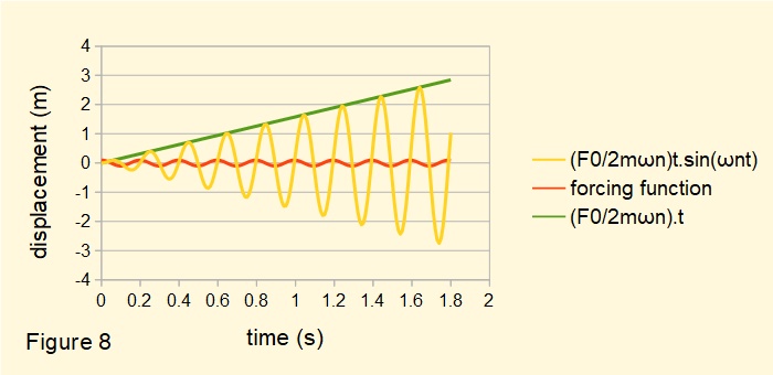
This plot shows the harmonic resonant response (yellow) induced by forcing function (red) F₀cos(ωt) for ω = ω_n implied by the steady state response for ω → ω_n illustrated in Figure 5 above.

Note that line (green) x(t) = (F₀ / 2mω_n).t expresses the increase in amplitude of the vibration. Note also the harmonic response sin(ω_nt) and forcing function cos(ω_nt) are out of phase by 90°.

Next:  Forced vibrations with damping

return to home page

I welcome feedback at:

alistair@alistairstutorials.co.uk