In previous tutorials expressions for internal shearing forces and bending moments for different beam support and loading conditions were derived from equations for static equilibrium. In this tutorial we demonstrate an alternative method for determining shearing forces V and bending moments M using singularity functions.
Singularity functions appear complex at first but once you understand the "rules" the method becomes clearer.
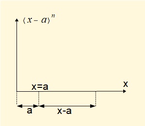
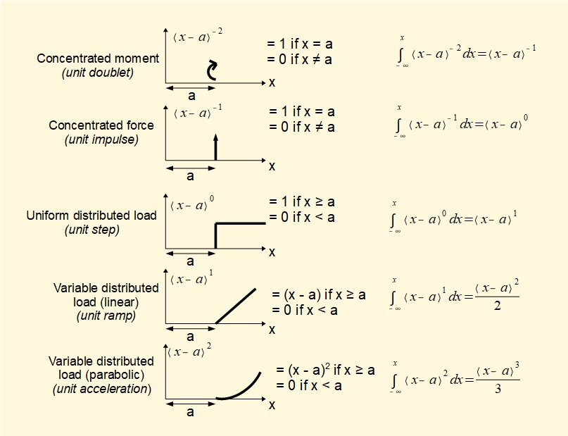
It must be understood that singularity functions are not normal algebraic expressions. They are conventionally enclosed within angle brackets < >. Singularity functions apply at discontinuities, such as load points and changes in load conditions along a beam. We define discontinuities occurring at points a on the x axis (see below). The singularity function is defined by the expression <x - a>n where the exponent n can be -ve, +ve or 0.
There are two sets of rules concerning singularity functions that we use:
- values of the function when x < a, x = a and x > a
- integrals of the function for specific values of the exponent n
These properties are defined below for the range of functions (i.e. the exponents) of interest to us. Note that a specific type of applied load is associated with each function: note also the formal generic name of each function (e.g. unit impulse).
We now define a loading function q(x) corresponding to each singularity function as follows:
- for an applied moment M (kNm) at x = a: q(x) = M<x - a>-2
- for a concentrated force F (kN) at x = a: q(x) = -F<x - a>-1
- for a uniformly distributed load w (kN/m) applied from x = a: q(x) = -w<x - a>0
- for a linear variable distributed load s (kN/m2) applied from x = a: q(x) = -s<x - a>1
Note that the signs for the above functions are valid for positive (clockwise) applied moments and negative applied forces and must be reversed where necessary (the example below will demonstrate this).
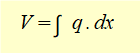
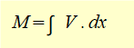
A loading function q comprising all moments and loads applied to the beam is then stated and expressions for V and M obtained using the following relationships.
We now demonstrate an example of the method using a simply supported beam with two point loads and a uniformly distributed load over a portion of the beam.
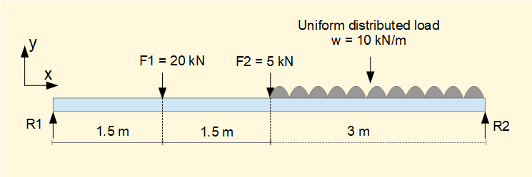
The equivalent point load of the distributed load w is 3w kN with centre of action at x = 4.5 m
To find R1 and R2:
(a) sum of forces = 0 (R1 and R2 are +ve forces; F1, F2, and w are -ve forces)
gives: R1 + R2 - F1 - F2 - 3w = 0 ------(i)
(b) sum of moments about x = 0 (clockwise moments are +ve)
gives: (6 x R2) = (3w x 4.5) + (F2 x 3) + (F1 x 1.5 ) = 135 + 15 + 30 = 180
Thus: R2 = (180)(/6) = 30 kN
From (i) R1 = F1 + F2 + 3w - R2 = 20 + 5 + 30 - 30 = 25
Thus: R1 = 25 kN
We now state the loading function q(x) for each load element in terms of the singularity function
<x - a>n where a is the value of x (as x increases along the beam) corresponding to: (a) the location of the point loads, (b) the initial point of loading for the distributed load.
giving for R1: q(x) = R1<x - 0>-1 (note R1 acts in the +ve direction - see comment above regarding sign)
giving for F1; q(x) = -F1<x - 1.5>-1
giving for F2: q(x) = -F2<x - 3>-1
giving for w: q(x) = -w<x - 3>0 (note a = 3 is the initial point of loading for the distributed load)
giving for R2 q(x) = R2<x - 6>-1
Thus the complete loading function is:
q(x) = R1<x - 0>-1 - F1<x - 1.5>-1 - F2<x - 3>-1 - w<x - 3>0 + R2<x - 6>-1 --------- (ii)

Thus integrating (ii) gives:
V(x) = R1<x - 0>0 - F1<x - 1.5>0 - F2<x - 3>0 - w<x - 3>1 + R2<x - 6>0 --------- (iii)
We can now evaluate each singularity function <x - a> in this expression using the rules defined above for x = a. Remember the value always = 0 for x < a.
which gives: <x - 0>0 = 1 <x - 1.5>0 = 1 <x - 3>0 = 1 <x - 3>1 = (x - 3) <x - 6>0 = 1
Note the change of notation from <x - 3>1 to algebraic notation (x - 3)
We now have an expression for V(x) as follows:
V(x) = R1 - F1 - F2 - w(x - 3) + R2 --------- (iv)
We use use this expression to form the shearing force diagram..
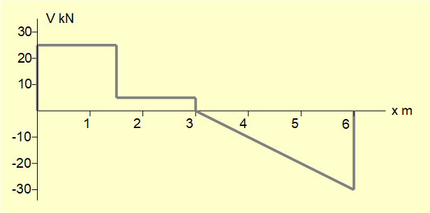
The diagram is composed as follows.
At x = 0 there is a step change of V = +R1 = 25 kN
The next "change point" is at F1. Thus from x = 0 to x = 1.5 V = R1 = 25 kN
At x = 1.5 there is a step change of V = -F1 = -20 kN
The next change point is at F2. Thus from x = 1.5 to x = 3 V = (25 - F1) = (25 - 20) = 5 kN
At x = 3 there is a step change of V = -F2 = -5 kN and a linear function V = -w(x - 3) = -10(x - 3) kN
The next change point is at R2. Thus from x = 3 to x = 6 V = [5 - (F2) - w(x - 3)] = [(5 - 5 -10(x - 3)] = (30 - 10x) kN. This is a linear function; note that where x = 3, V = 0 and where x = 6, v = -30 kN
At x = 6 there is a step change of V = +R2 = 30 kN and a linear function (30 - 10x).
Thus at x = 6 V = [R2 + (30 - 10x)] = [30 + (30 - 60)] = 0 which is the expected result for the loading condition at x = 6.

From (iii) above
V(x) = R1<x - 0>0 - F1<x - 1.5>0 - F2<x - 3>0 - w<x - 3>1 + R2<x - 6>0
Integrating gives:
M(x) = R1<x - 0>1 - F1<x - 1.5>1 - F2<x - 3>1 - w<x - 3>2/2 + R2<x - 6>1 --------- (v)
Again we evaluate each singularity function <x - a> in this expression using the rules defined above for x = a. Remember the value always = 0 for x < a.
which gives: <x - 0>1 = x <x - 1.5>1 = (x - 1.5) <x - 3>1 = (x - 3) <x - 3>2/2 = (x - 3)2/2
<x - 6>1 = (x - 6)
note the change to algebraic notation for functions of x
We now have an expression for M(x) as follows:
M(x) = R1.x - F1(x - 1.5) - F2 (x - 3) - w(x - 3)2/2 + R2(x - 6) -------- (vi)
We use use this expression to form the bending moment diagram.
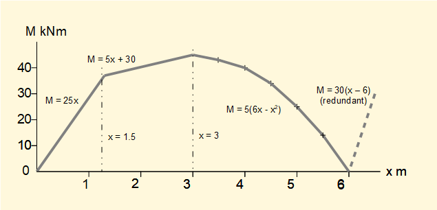
The diagram is composed as follows.
From x = 0 to x = 1.5 there is a linear function M(x) = (R1)x = 25x
From x = 1.5 to x = 3 there is a linear function M(x) = [(25x} - F1(x - 1.5)]
giving: M(x) = [(25x) - 20(x - 1.5)] = (5x + 30)
From x = 3 to x = 6 there is a quadratic function M(x) = (5x + 30) - F2(x - 3) - w(x - 3)2/2
giving: M(x) = 5x +30 - 5(x - 3) - 10(x - 3)2/2
giving: M(x) = [5x + 30 - 5x + 15 - 5x2 +30x - 45] = [30x - 5 x2 ] = 5(6x - x2 )
At x = 6 the function M(x) = R2(x - 6) = 30(x - 6) applies but this function makes no tangible contribution to the bending moment as non-zero values are beyond the physical extent of the beam.
Next: Normal bending stresses in beams
I welcome feedback at: