Crank mechanism - crank effort and balancing

This tutorial concerning slider and crank mechanisms covers two aspects directly related to the operation of actual machines.

We look firstly at output characteristics of a crankshaft and flywheel under torque load conditions using crank effort diagrams. We then consider balancing of inertial forces and moments generated in the mechanism.

Crank effort

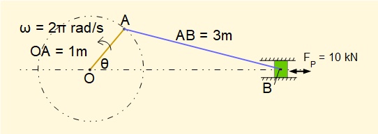
Consider the crank mechanism as an engine operating at constant angular velocity ω against a constant torque load. We use the mechanism with parameters from previous tutorials shown below but with the driving force increased by a factor of 10 to the more practical value of 10 kN. The horizontal driving force F_P at the slider is constant and "double acting", i.e. the direction of the force reverses at θ = 180°.

The plot below, called a crank effort diagram, shows the fluctuating torque generated by the engine at the crankshaft, called the engine torque, over one rotational cycle, derived from first principles shown in a previous tutorial. For simplicity we ignore the effects of inertia forces and moments.

Work done by engine torque = \(\large\int\limits_{0}^{2\pi}T\,d\theta\)  where T is a function of θ.

Thus the area under the engine torque plot is the work done in one crank cycle which we calculate by numerical integration to be 39 900 Nm. Constant angular velocity ω = 2π rad/s is equivalent to one crank cycle per second giving the power output (rate of work) = 39.9 kW.

We represent the same amount of work being done by a constant torque T_av called the mean engine torque. T_av = 39 900/2.π = 6350 Nm as shown on the plot.

T_av is also the constant load torque on the engine running at nominally constant angular velocity ω. Given the highly fluctuating engine torque how can constant (or near constant) angular velocity be maintained? The answer is by the rotational inertia of a flywheel and other rotating masses with rotational inertia in the drive chain.

Referring to the crank effort diagram above, where engine torque is greater than T_av the engine provides energy to the flywheel which increases ω. Conversely, where engine torque is less than T_av the flywheel provides energy to the engine which causes ω to reduce Thus ω fluctuates between upper and lower values over one cycle.

We now estimate the variation in ω occurring with a flywheel having mass moment of inertia I_F.

Let the highest and lowest angular velocities of the flywheel be respectively ω_max and ω_min

Consider the diagram below. From the crank effort diagram we identify which segment of the cycle has the maximum fluctuation in energy E_FL relative to the mean engine torque. From numerical integration we establish that segment B has the largest fluctuation of E_FL = 5910 Nm . Thus ω_max occurs at the transition point between segments A and B and ω_min at the transition between segments B and C.

From first principles    \(\large E_{FL} = \frac 1 2 I_F (\omega_{max}^2 - \omega_{min}^2) \)

Giving    \(\large E_{FL} = \frac 1 2 I_F (\omega_{max} + \omega_{min})(\omega_{max} - \omega_{min})\)

If the variation in speed is small    \(\large(\omega_{max} + \omega_{min}) \approx 2\omega\)

Giving    \(\large E_{FL} = \frac 1 2 I_F 2 \omega (\omega_{max} - \omega_{min}) = I_F\omega (\omega_{max} - \omega_{min})\)

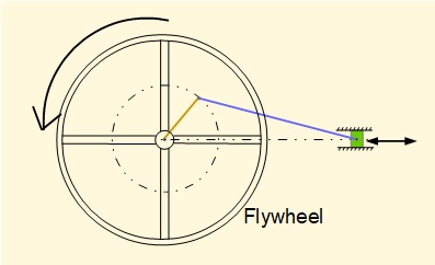
In the following practical example we attach to the crankshaft a spoked annular ring flywheel shown below, twice the diameter of the crank arm with mass moment of inertia I_F = 6000 kgm².

For ω = 2π rad/s and E_FL = 5910 Nm (from above) we can find (ω_max - ω_min) :

\(\large(\omega_{max} - \omega_{min}) = {\Large E_{FL}\over I_F\omega}\)

Giving  (ω_max - ω_min) = 0.157 rad/s (1.50 rev/min).

The following ratios are commonly stated:

\(\LARGE(\omega_{max}-\omega_{min})\over\omega\)    known as the coefficient of fluctuation of speed

\(\Large E_{FL} \over work~done~per~cycle\)   known as the coefficient of fluctuation of energy

In example above the coefficient of fluctuation of speed = 0.025 (2.5%) and the coefficient of fluctuation of energy = 0.148 (14.8%). These are typical values for double acting, single cylinder steam engines (such as they exist now!).

However this high degree of control over output speed comes at a cost as the flywheel in this example has a large mass (c.1500 kg) and the high mass moment of inertia makes the engine difficult to start from rest.

To achieve the same output with a smaller flywheel we now consider three identical engines with the crank arms 120° apart on the same crankshaft and the driving force F_P at each engine = 3.33 kN. The crank effort diagram below shows the effect.

To achieve the same mean engine torque and coefficient of fluctuation of speed with a smaller flywheel we now consider three identical engines with the crank arms 120° apart on the same crankshaft and the driving force F_P at each engine = 3.33 kN. The crank effort diagram below shows the effect.

The mean engine torque is unchanged but the maximum fluctuation of energy E_FL by numerical integration = 1732 Nm giving a coefficient of fluctuation of energy = 4.3% as opposed to 14.8% for a single crank.

The same coefficient of fluctuation of speed = 2.5% is achieved with a flywheel having mass moment of inertia = 1755 kgm² with a corresponding reduction of mass to 461 kg (for identical dimensions of the flywheel in the plane of rotation)

The example above is simple based on an idealised engine. Crank effort diagrams for real engines where piston pressures vary throughout the working stroke are significantly more complex.

Balancing

In a previous tutorial we examined inertia forces and moments generated in a slider and crank mechanism and estimated their effect on crankshaft torque and reaction forces at bearings. Fluctuating forces associated with inertial effects can generate vibrations which are transmitted to the machine supports. Measures to neutralise these effects are known as balancing.

Firstly, a brief summary of the basic principles of balancing.

Static balance

The diagram below illustrates the principle of static balance.

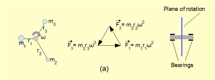
In diagram (a) masses m_i are attached by massless rods of radius r_i to a shaft rotating with angular speed ω. The centripetal acceleration r_iω² of each mass is associated with a longitudinal tension force in each rod = m_ir_iω² and corresponding reaction forces on the shaft bearings. In this case the sum of these force vectors is zero thus there is no resultant reaction force at the shaft bearings arising from rotation. In this state we say that the rotating shaft is in static balance. The general requirement for static balance of rotating masses is Σm_ir_i = 0 (considering r as a vector). The term static is appropriate since the rotor is in static equilibrium at all angular positions of the shaft.

This condition can also be expressed by saying that the vector sum of the centrifugal inertial forces* for the masses is zero.

* The longitudinal tension force in the rod accounts for the centripetal acceleration of the rotating mass directed towards the centre of rotation The diagram above shows the reaction force of this tension acting on the rotating masses. Centrifugal inertial forces acting on the masses, directed away from the centre of rotation, are "pseudo forces" which allow analysis of rotating masses using the condition of static equilibrium. ( D'Alembert's principle - see previous tutorial). It is conventional to show centrifugal forces in diagrams illustrating balancing (see below).

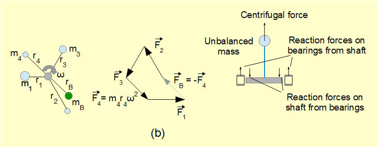
In diagram (b) an additional mass m₄ is attached to the rotor. Now the vector sum of tension forces in the rods is not zero. The rotor is in a state of static unbalance and a net force arises on the rotor shaft bearings. In this example the unbalanced force F₄ = m₄.r₄.ω². A balancing mass m_B can be added to restore static balance such that m_B.r_B.ω² = -m₄.r₄.ω².

Dynamic balance

The diagram below illustrates the principle of dynamic balance.

In the diagram above a rotor shaft mounted on bearings A and B with attached masses of equal mass m at radius of rotation r is shown at angles of rotation 0° and 180°. The rotor meets the condition for static balance as Σm_ir_i = 0 for all angles of rotation.

Using statics we calculate reaction forces from the bearings on the rotor shaft at bearing positions A and B for angle of rotation = 0° arising from centripetal acceleration m.ω².r of each mass m.

Sum of vertical forces = 0:

R_B + m.ω².r - R_A - m.ω².r = 0

gives:    R_A = R_B

Sum of moments about bearing position A = 0:

6.R_B + 1.m.ω².r - 5.m.ω².r = 0

gives:    6.R_B = 4.m.ω².r    gives:    R_B = R_A = 2.m.ω².r/3

It is clear that the directions of forces reverse 180° at angle of rotation = 180°.

The rotor is in a state of dynamic unbalance where centrifugal inertial forces mω²r exert a moment on the shaft with resultant rotating reaction forces on the bearings. Location of the rotating masses along the axis of the shaft determines the magnitude of the bearing forces, the further apart the rotational planes the larger the forces. In the limiting case when the rotating planes converge, reaction forces are zero.

Dynamic balancing involves placing additional mass on the rotor at positions such that the net moment on the shaft is zero. It is particularly important in the design of multi-cylinder engines. In this tutorial we examine only static unbalance generated in a single crank arrangement.

Balancing a slider and crank mechanism

In a previous tutorial we identified inertial forces generated by the three moving elements of a slider and crank mechanism:

• Rotational inertial force generated by the crank arm


• Reciprocating (translational) inertial force generated by the slider


• Inertial force and moment generated by the connecting rod

We examine balancing these inertial forces and moments from each element in turn using the example mechanism below.

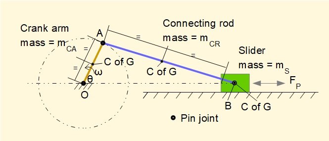
Individual elements are as follows. The C of G is located at the mid-point of each element.

• Mass of slider m_S = 10 kg


• Mass of connecting rod m_cr = 5 kg


• Mass of crank arm m_ca = 2 kg


• Length of connecting rod L = 3 m


• Length of crank arm R = 1 m


• Angular velocity of crank arm ω = 2π rad/s


• Crank angle θ : in this example θ = 50°

Balancing rotation of the crank arm

Referring to the diagram below the inertial centrifugal force F_Ica experienced by the crank arm rotating at constant angular velocity ω produces a rotating unbalanced force acting through point O. In this example the C of G of the crank arm is at position R/2. Thus F_Ica = m_caω²(R/2) = 2 x (2π)² x 0.5 = 39.5 N

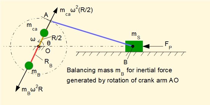
We can balance this force by placing a rotating counterbalance mass m_B at radius R_B diametrically opposed to the crank arm such that m_B x R_B = m_ca x (R/2) giving for this example m_B = 1/R_B kg

Balancing reciprocal motion of the slider

Acceleration a_B of the reciprocating slider of mass m_S produced by applied force F_P generates an inertial force F_IS such that F_IS = - (m_S x a_B)*

*negative sign indicates that the "pseudo" inertial force opposes the direction of the acceleration vector.

In a previous tutorial we derived the following expression for the acceleration of the slider, a_B

In this previous tutorial we derived the above expression for a_B by successive differentiation of the linear displacement of point B as a function of crank angle θ. When considering balancing it is convenient to express the second term in brackets as follows*.

* This approximation is obtained by applying the binomial theorem to the expression for displacement of point B.

We now consider the inertial force generated by the slider as two separate parts:

Primary inertia force

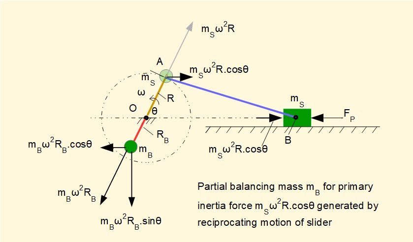
The diagram above shows the primary inertia force m_Sω²Rcosθ generated by the acceleration of mass m_S at crank angle θ = 50°. This force varies in magnitude and direction through the complete crank cycle as a function of cosθ.

In this example at θ = 50° this force = 10 x (2π)² x 1 x 0.64 = 253 N. The maximum value of the primary force component (at θ = 0° and 180° ) = 10 x (2π)² x 1 x 1 = 395 N.

This force can be seen as equivalent to the horizontal component of the centrifugal force generated by an imaginary mass m_S rotating about point O at radius R which can be balanced by the horizontal component of the centrifugal force generated by a diametrically opposed counter-balance mass m_B at radius R_B such that (m_B x R_B) = (m_S x R).

However, the vertical component of the centrifugal force generated by the counter-balance mass m_B creates an unbalanced force = m_Bω²R_Bsinθ. In practical terms it is a question whether suppression of an oscillating force in in the horizontal plane outweighs the adverse effect of creating an oscillating force in the vertical plane. A partial balance of the primary component between 50% and 65% is commonly applied.

Secondary inertia force

which is a function of cos2θ and can be interpreted as the horizontal component of the centrifugal force generated by an imaginary mass m_S rotating on a secondary imaginary crank arm with angular velocity 2ω rad/s such that:

Thus the radius of this secondary crank = R/4n. This force can be balanced by counter-balance mass m_B on a diametrically opposed secondary crank arm at radius R_B such that m_S x (R/4n) = m_B x R_B as shown in the diagram below. In common with the counter-balance for the primary inertia force this method of balancing introduces an unbalanced vertical force = m_B(2ω)²R_Bsinθ.

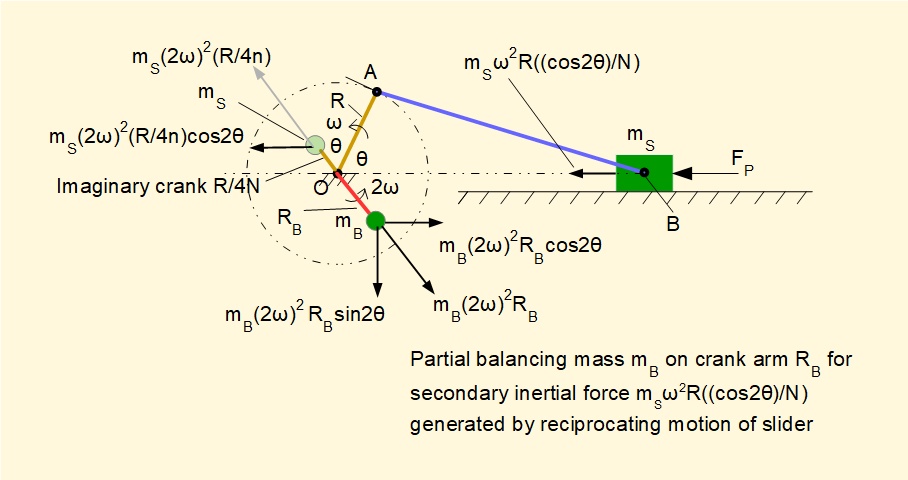
The difficulty of constructing a practical arrangement for a secondary crank is such that balancing the secondary inertia force is generally restricted to multiple-cylinder internal combustion engines where secondary reciprocating inertia forces can be significant.

Balancing inertial forces and moments in the connecting rod

In a previous tutorial we examined the inertial force and moment generated by the connecting rod shown in the diagram below for a specific crank angle θ.

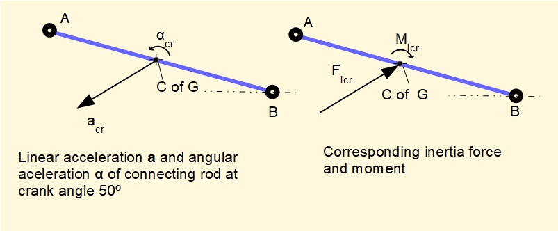
We now convert this inertia force and moment to an equivalent dynamical system representing the total mass of the connecting rod m_cr as two point masses m₁ and m₂ conveniently located at points B and A connected by a massless link as shown below. We then add the inertial forces generated by m₁ and m₂ respectively to the inertial forces generated by the slider and crank arm.

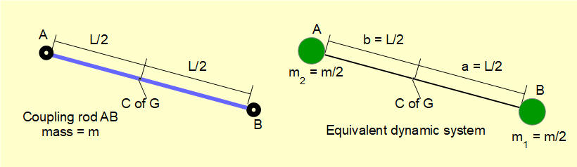
The general criteria for an equivalent dynamic system with reference to the parameters of the right hand diagram above are:

1. m_cr = m₁ + m₂


2. m₁.a = m₂.b


3. m₁.a² + m₂.b² = m.k²    where k is the radius of gyration of the component rotating about an axis through its centre of gravity

For the case above where m₁ = m₂ = m_cr/2 and a = b = L/2 it is clear that criteria #1 and #2 are satisfied.

To test for criterion #3:

m₁.L²/4 + m₂.L²/4 = (m₁ + m₂).L²/4 = m.(L²/4)

For a slender rod rotating on an axis through its C of G, k = L//√12 giving m.k² = m.(L²/12)

Clearly criterion #3 is not satisfied*¹ with this arrangement of masses*². However, the partial dynamic equivalence defined above where m₁ = m₂ = m_cr/2 provides an approximate measure of the unbalance generated by the inertia of the coupling rod.

*¹ Complete dynamic equivalence can be obtained by applying a "correction couple" = m.(a.b - k²).α where α is the angular acceleration of the connecting rod. Since α varies continuously the correction has limited value for the purpose of determining any counter-balancing mass.

*² An equivalent dynamic system satisfying all three conditions with one mass located at point A or point B and the other mass located elsewhere on the rod axis does exist but this arrangement of masses does not suit our purpose in terms of balancing. A procedure to establish an equivalent dynamical system without a correction couple is outlined in a previous tutorial.

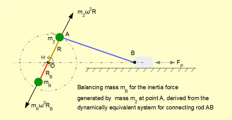
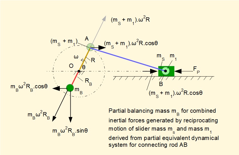
The diagrams below show masses m₂ and m₁ incorporated into balancing masses m_B for:

• inertia forces associated with rotation of the crank arm


• inertia forces associated with reciprocating motion of the slider

Next:  Crank mechanisms - offsets and eccentrics

return to home page

I welcome feedback at:

alistair@alistairstutorials.co.uk