Crank mechanism - inertia forces and crankshaft torque

In a previous tutorial we examined action and reaction forces generated in the elements of a slider and crank mechanism by using free body diagrams for an engine and a compressor. In this tutorial we expand free body diagrams to include inertia forces and inertia torques generated in the individual elements (slider, connecting rod and crank arm), a general topic known as kinetics. We also consider several different methods of calculating the torque produced at the crankshaft of an engine delivering power through a crank mechanism.

Inertia forces and torques

Overview

The following free body diagrams illustrate the concepts of inertia forces and torques.

(note: the terms inertia torque and inertia moment are synonymous)

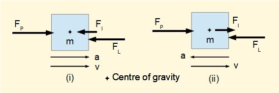
arrows v and a illustrate directions of velocity and acceleration vectors for mass m.

In diagram (i) F_P is the force which must be applied to accelerate mass m at a m/s² against constant load force F_L (ignoring friction). The force required to produce this acceleration is F_a = m.a. We say the inertia of mass m "resists acceleration" through a "pseudo" inertia force F_I which is equal and opposite to F_a and acts through the centre of gravity. We then use D'Alembert's principle to treat accelerating masses as if they are in static equilibrium by incorporating inertia forces and moments. Thus in our example with the inertial force F_I and the sum of forces = 0 ("pseudo" equilibrium condition) gives
F_P = F_L + F_I. However, the true net force on mass m is F_a = F_P - F_L (not in equilibrium because the mass is accelerating).

By contrast, in diagram (ii) force F_P must be applied to decelerate mass m against the same constant load force F_L with acceleration = -a. The inertia force F_I now acts in the opposite direction resisting deceleration. In this case sum of forces = 0 gives F_P = F_L - F_I.

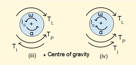
Diagrams (iii) and (iv) show the inertia torques T_I when torque T_P is applied to a counter-clockwise rotating mass with mass moment of inertia I_G against a constant load torque T_L with angular acceleration α radians/sec². The torque T_α required to produce angular acceleration α = I_G.α and the reactive inertia torque T_I is equal and opposite. In diagram (iii) (counter-clockwise α ) T_P = T_L + T_I. In diagram (iv) (clockwise α) T_P = T_L - T_I.

note: the convention in mechanics is that counter-clockwise rotations are positive and clockwise rotations negative.

Inertia forces and torques in a slider and crank mechanism

We use of inertia forces and moments to take account of forces in the crank mechanism associated with acceleration of masses.

The analysis requires that inertia forces and moments act through or about the centre of gravity of the moving elements. We begin by determining the mass and centre of gravity of each element for the example shown below.

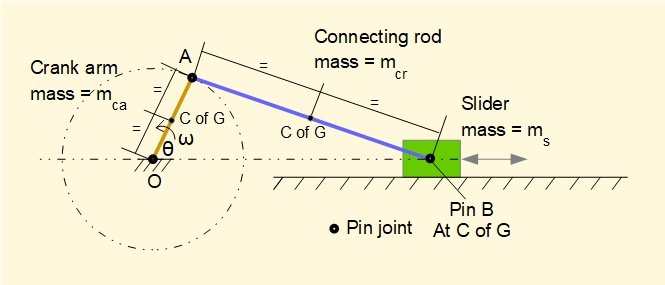
For simplicity we assume the crank arm and connecting rod have uniform cross section along their length, thus centres of gravity are at the mid-points.

We will identify the inertia forces and moments generated by accelerations of the individual elements and then illustrate with a numerical example.

Inertia of the crank arm

In this example we restrict the analysis to a crank arm rotating with constant angular velocity ω, thus the crank arm has no angular acceleration and correspondingly no inertia torque. We take account of the centripetal acceleration of point A directed radially towards centre of rotation O when considering connecting rod AB.

Inertia of the slider

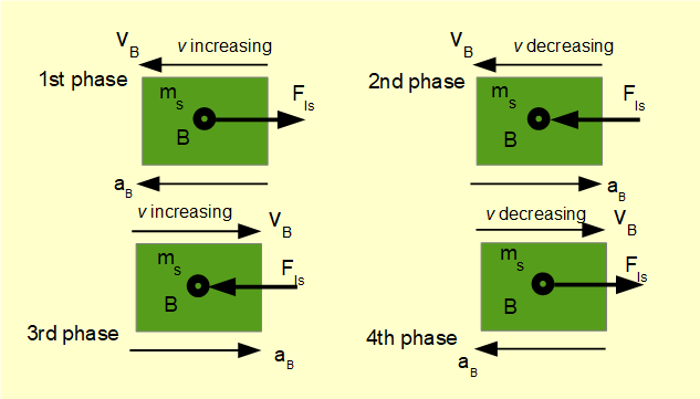
We established in an earlier tutorial that the slider experiences linear acceleration which varies constantly throughout the crank cycle. There are four distinct phases in the cycle when the absolute slider velocity is increasing or decreasing. In the diagram below we show the direction of inertia forces F_Is for each phase of the crank cycle. For a horizontal slider the first phase starts at the inner dead centre position (crank angle ω = 0°). The transition between second and third phases occurs at outer dead centre (crank angle ω = 180°). Crank angles for the other two transitions depend on ratio of connecting rod and crank arm lengths (n).

In all cases F_Is = m_s.a_B

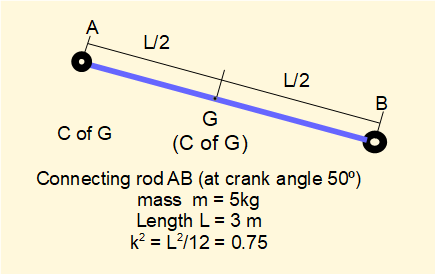
Inertia of the connecting rod

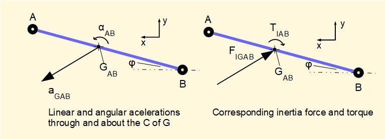
To determine the inertia forces generated by the mass of the connecting rod we require: (i) the linear acceleration of the centre of gravity (point G_AB) relative to point O which we designate a_GAB, (ii) the inertia moment of AB about point G_AB which we designate T_IAB = I_g.α_AB where I_g is the mass moment of inertia about point G_AB and α_AB is the angular acceleration of AB.

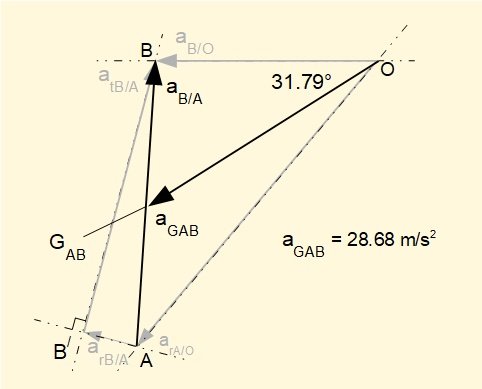
To obtain a_GAB we use the acceleration diagram developed in a previous tutorial shown below. Note this diagram is specifically for crank angle ω = 50°.

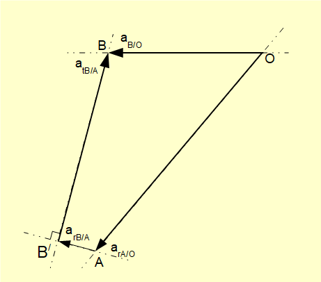
To recap, accelerations shown on this diagram are:

• a_rA/O the acceleration of point A relative to point O in a radial direction along crank arm AO. Because angular velocity ω of the crank arm is constant in this example there is no tangential component of acceleration of A relative to O.


• a_rB/A the acceleration of point B relative to point A in a radial direction along connecting rod AB.


• a_tB/A the acceleration of point B relative to point A tangential to connecting rod AB.


• a_B/O the acceleration of point B relative to point O, which is the linear acceleration of the slider mass considered above.

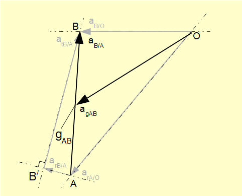
To develop this acceleration diagram to find a_GAB (see below) firstly show the acceleration of point B relative to point A, a_B/A which is the sum of radial and tangential components. In our example the acceleration at point G_AB is at the mid-point of this line corresponding to the position of the centre of gravity of the connecting rod. Thus line OG_AB represents a_GAB. This acceleration is the absolute value relative to ground point O and is opposed by inertia force F_IGAB = m_cr.a_GAB acting through point G_AB, where m_cr is the mass of the connecting rod.

To find the inertia moment about point G_AB designated T_IAB = I_g.α_AB we proceed as follows.

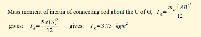
The mass moment of inertia I_g of a slender bar about its centre of gravity = m.L²/12 where m is the total mass and L the length.

α_AB = (a_tB/A )/AB is obtained from the acceleration diagram.

The diagram below illustrates the inertia force and inertia torque acting on the connecting rod for crank angle θ = 50°.

The inertia force and torque result in reaction forces at pin joints A and B. The object of the following numerical example is to find these reaction forces.

Example

The physical parameters of the crank mechanism in the example, shown below, are the same as the examples in the kinematics tutorials. In this idealised arrangement the load torque on the crank arm varies such that the angular velocity ω remains constant through a complete crank cycle while maintaining a constant force F_P on the slider. We also ignore the effects of friction.

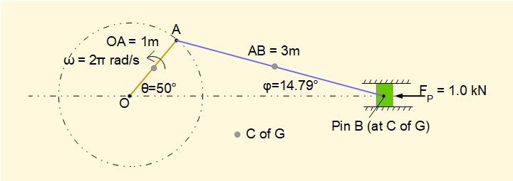
Individual elements have the following mass. The C of G is located at the mid-point of each element.

• Mass of slider (m_s) = 10 kg


• Mass of connecting rod (m_cr) = 5 kg


• Mass of crank arm (m_ca) = 2 kg

Force F_P = 1.0 kN is applied to the slider in the direction shown (for crank angles > 180° the direction of F_P reverses)

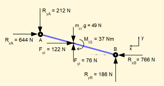
A free body diagram of connecting rod AB is shown below for crank angle = 50°. We use sum of forces in x direction = 0, sum of forces in y direction = 0 and moments about C of G = 0 to find the unknown reaction forces.

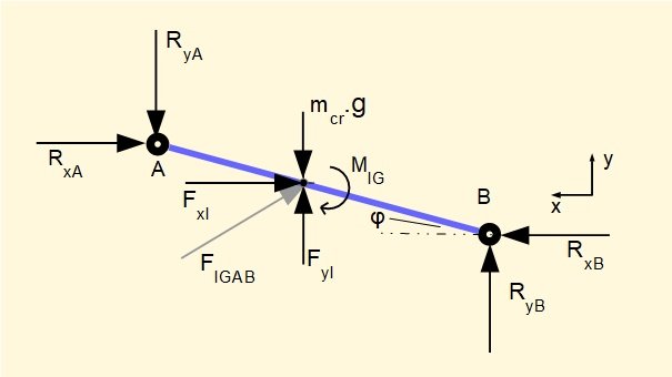
F_xI and F_yI are the x and y components of inertia force F_IGAB

R_xB is the horizontal reaction force exerted on B by the slider and acts in a +ve direction on the x axis. We reasonably deduce that the horizontal reaction force at point A, R_xA, acts in the -ve direction. We also reasonably deduce that the vertical reaction forces R_yB at point B and R_yA at point A will be +ve and -ve respectively on account of the direction of thrust along the connecting rod.

M_IG is the inertia moment about the C of G.

m_cr.g is the gravity force of the connecting rod acting vertically down through the C of G.

As a first step we obtain the value of R_xB from the free body diagram for the slider (below) where R_xB is the equal and opposite reaction force on the slider.

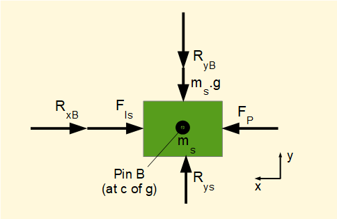
The inertia force on mass m_s is F_Is = m_s.a_B where a_B is the linear acceleration of point B. From a previous tutorial we know for this mechanism and crank angle θ = 50° that a_B = 23.4 m/s². Note in passing that reaction force R_yB on the slider from the connecting rod is opposed by reaction force R_ys from the cylinder wall. This vertical reaction force also opposes gravity force m_s.g.

For sum of horizontal forces on the slider = 0:

F_P - F_Is - R_xB = 0     Hence R_xB = F_P - F_Is

We now calculate inertia force F_IGAB acting on the connecting rod through its C of G. From the acceleration diagram below derived in a previous tutorial for this mechanism we obtain by geometry the value of a_GAB and its direction relative to the horizontal axis.

Referring to the free body diagram for the connecting rod above the inertia forces through the Cof G are:

F_xI = m_cr x a_GAB x cos(31.79°) = 5 x 28.68 x cos(31.79°) = 121.9 N

F_yI = m_cr x a_GAB x sin(31.79°) = 5 x 28.68 x sin(31.79°) = 75.5 N

For sum of horizontal forces on connecting rod = 0:

R_xB - F_xI - R_xA = 0    gives: R_xA = R_xB - F_xI    gives: R_xA = 766 - 121.9 = 644.1 N

For sum of vertical forces on connecting rod = 0:

F_yI - R_yA - m_cr.g + R_yB = 0    gives: R_yA - R_yB = F_yI - m_cr.g    gives: R_yA - R_yB = 75.5 - (5 x 9.81)

gives:    R_yA - R_yB = 26.5 N

For sum of moments about C of G of connecting rod = 0 (counter-clockwise moments +ve):

R_yA x 1.5 x cos(14.79°) - R_xA x 1.5 x sin(14.79°) + R_yB x 1.5 x cos(14.79°) - R_xB x 1.5 x sin(14.79°) - M_IG = 0

M_IG = I_g x α_AB and from a previous tutorial for this mechanism we know α_AB = 9.91 rad/sec2

Substitute R_yA = 26.5 + R_yB   gives:

(26.5 + R_yB) x 1.5 x cos(14.79°) - 644.1 x 1.5 x sin(14.79°) + R_yB x 1.5 x cos(14.79°) - 766 x 1.5 x sin(14.79°) - (3.75 x 9.91) = 0

gives:   38.4 + 1.45 x R_yB - 246.6 + 1.45 x R_yB - 293.3 - 37.2 = 0

gives:   2.9 x R_yB = 538.7    gives: R_yB = 185.8 N   and   R_yA = 185.8 + 26.5 = 212.3 N

The completed free body diagram for the connecting rod is shown below. Values are rounded to whole numbers.

It should be emphasised again that inertia moments and forces vary continuously throughout the cycle of the crank mechanism. This example is a snapshot at crank angle = 50° where inertia forces oppose the driving force and consequently reduce the torque available at the crankshaft. At other points in the cycle inertia forces aid the driving force and increase the crankshaft torque. In the next section we look at crankshaft torque in more detail.

Crankshaft torque

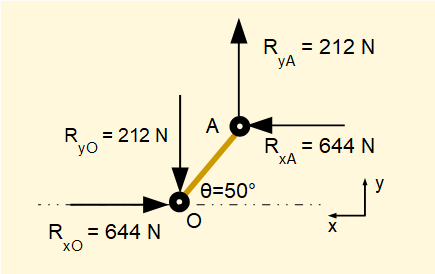
Crank arm AO = 1.0 m

Gives crankshaft torque T_cs = R_xA x 1.0 x sin(50°) + R_yA x 1.0 x cos(50°) = 644 x sin(50°) + 212 x cos(50°) = 630 Nm

Note: the complete free body diagram representing static equilibrium for the crank arm would include a clockwise moment about point O equal in magnitude to T_cs.

Crankshaft torque - alternative method

This is an example of the graphical methods traditionally used to determine kinematic and kinetic properties of crank mechanisms. Values to an acceptable tolerance would normally be obtained directly from scaled drawings.

Consider the diagram below derived in a previous tutorial showing velocities relative to ground point O of slider B (v_B) and crank pin A (v_A) and construction of the velocity pole for connecting rod AB.

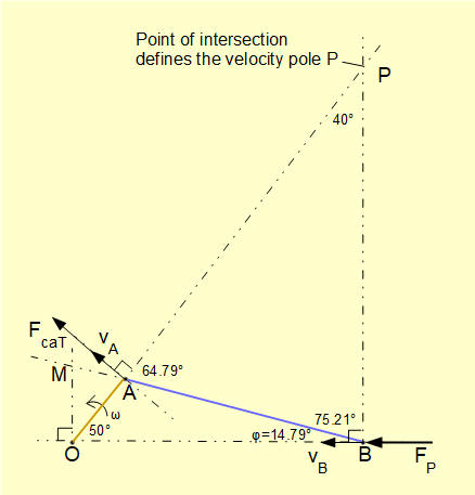
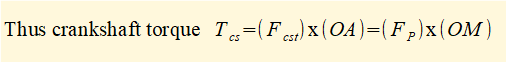
Now add to this diagram the external horizontal force F_P applied to the slider and the resultant force F_cst at crank pin A perpendicular to crank arm OA which delivers torque T_cs to the crankshaft such that T_cs = F_cst.OA

Using the principle that the rate of work done at point B must equal the rate of work done at point A it follows that:

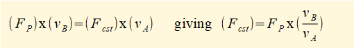
From the diagram it follows from the definition of velocity pole point P that: v_B = PB x ω_AB and v_A = PA x ω_AB where ω_AB is the angular velocity of connecting rod AB.

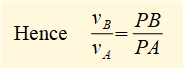
Now on the velocity pole diagram extend line BA and take a perpendicular line from point O to intersect extended line BA at point M forming triangle AOM. Triangles APB and AOM are similar such that:

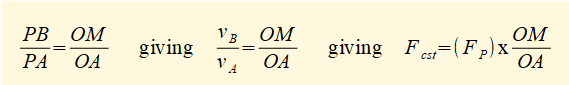
In this example OM is calculated from the extended velocity pole diagram above by simple geometry giving the value OM = 0.93 m.

We defined F_P as the external force on the slider which in the previous example = 1 kN, giving the crankshaft torque by this method T_cs = 1000 x 0.93 = 930 Nm compared to 630 Nm from the previous calculation.

This method gives a first approximation of crankshaft torque excluding inertia forces and torques for the slider and connecting rod and gravity forces.

A better approximation of crankshaft torque takes account of the inertia force generated by the slider mass. From the previous example the net horizontal reaction force at B taking account of this inertia force is R_xB = 766 N, giving T_cs = 766 x 0.93 = 712 Nm. The remaining discrepancy is accounted for by the inertia force and inertia torque generated by the connecting rod and the gravity force of the rod.

Variation of crankshaft torque with crank angle

For convenience we used a crank angle = 50° for the above examples but crankshaft torque varies continuously throughout the full crank cycle. In previous tutorials we developed general expressions for velocities and accelerations of elements in the mechanism. For crankshaft torque there is a very convenient general expression derived from the velocity pole diagram (see above) where we noted that:

* previous tutorial

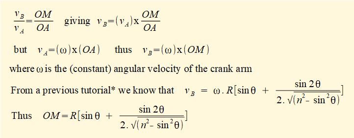
The diagram below plots crankshaft torque Tcs against crank angle using the above formula for the parameters applied in the previous examples. The diagram shows a full cycle for crank angle θ from 0° to 360° with the direction of the external force F_p = 1 kN on the slider reversed at θ = 180°. One plot shows crankshaft torque ignoring inertia forces the other shows the effect of the inertia force associated with acceleration of the slider mass only. The cyclical subtractive and additive effect of the inertia force is clear.

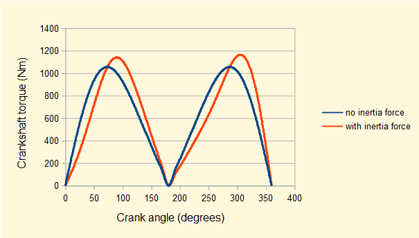
In a real engine the torque delivered to the load is smoothed by the rotational energy of a flywheel which cyclically transfers energy to and from the crank mechanism resulting in a relatively smooth "mean torque " in continuous operation. We look at this aspect in another tutorial.

Inertial forces on the connecting rod using equivalent dynamical systems

As shown above the contribution of inertia force and inertia moment acting on the connecting rod with respect to crankshaft torque can be computed using free body diagrams and equations using D'Alembert's principle. Other methods for determining crankshaft torque often use the principle of equivalent dynamical systems to account for the inertial effects of the connecting rod.

For an explanation of an equivalent dynamical system consider the following.

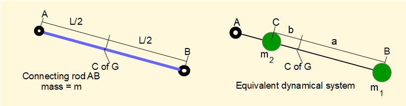
Connecting rod AB of mass m can be replaced by two point masses m₁ and m₂ located on AB at distances a and b relative to the centre of gravity according to the following requirements:

• m = m₁ + m₂ ------ (1)
• m₁ . a = m₂ . b ------ (2)
• m₁ . a² + m₂ . b² = m.(k_eq)² ------ (3)   

where: k_eq is the radius of gyration of the two equivalent masses rotating about an axis through the centre of gravity of the connecting rod and k_eq = k_cr where k_cr is the radius of gyration of the connecting rod itself rotating about an axis through its centre of gravity.

A procedure for setting valid parameters m₁, m₂, a and b is as follows:

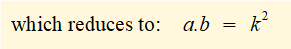
(Note this a general relationship between radius of gyration k for two concentrated masses linked by a massless rod rotating about a perpendicular axis where a and b are the respective distances of the masses from the axis of rotation. We will use this relationship in the section below for an equivalent dynamical system where condition (3) above does not apply.)

Now choose a position for m₁ at distance a from the centre of gravity, for example at point B in the diagram above. Point C on the rod must now be located distance b = k²/a from the centre of gravity.

m₁ and m₂ are then determined from (4) above.

We can now develop an equivalent dynamical system for the connecting rod in the example mechanism used in this tutorial.

A favourable position for mass m₁ is the rod/slider pin joint at point B. Thus a = 1.5 m.

Mass m₂ must be located at point C at distance b = k²/a from point G. Thus b = 0.75/1.5 = 0.5 m.

And then from (4) above: m₁ = 1.25 kg and m₂ = 3.75 kg.

The equivalent dynamical system is shown below with masses m₁ and m₂ represented in scale.

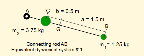
This arrangement is generally applied in graphical methods for determining kinematic and kinetic properties of crank mechanisms using Klein's diagram, commonly found in traditional text books for mechanics of machines.

Alternative arrangement for position of masses

Another arrangement for an equivalent dynamical system places m₁ and m₂ at the crank pin and rod/slider pin joint.

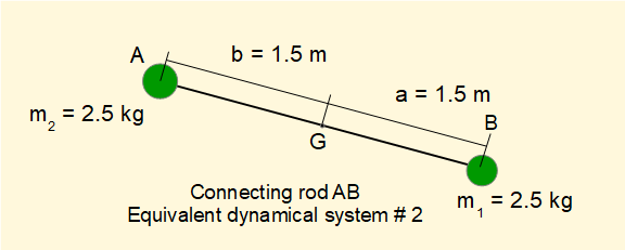
The arrangement shown meets requirements of (1) and (2) above.

Regarding condition (3):   m₁.a² + m₂.b² = m.(k_eq)² where (k_eq)² = a.b = 2.25 m².

From above:   (k_cr)² = L²/12 = 0.75 m².

Hence k_eq ≠ k_cr and requirement (3) is not met. This is resolved by applying a correction couple determined as follows.

Let T_cr be the torque derived from angular acceleration of the connecting rod α .

Thus:   T_cr = I_cr.α   where I_cr = m.(k_cr)²

Let T_eq be the torque also derived from angular acceleration α.

Thus:   T_eq = I_eq.α   where I_eq = m.(k_eq)² = m.a.b

It follows that a correction couple M_cor must be applied to the system where:   M_cor = T_cr - T_eq

Giving:   M_cor = m.[a.b - (k_cr)²].α

The direction of the correction couple is determined as follows:

if (k_eq)² > (k_cr)²   M_cor has the same rotational direction as α (the case in this example).

if (k_eq)² < (k_cr)²   M_cor has the opposite rotational direction to α

Forces generating torque at the crankshaft acting on masses m₁ at point B and m₂ at point A for this equivalent dynamical system are shown below.

Note this is not a conventional free body diagram. Paired action and reaction forces are omitted. The break in the connecting rod represents an arbitrary point for transmission of forces through the massless rod.

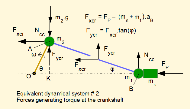
The correction couple M_cor resolves as a pair of vertical forces N_cc acting at points A and B where
N_cc.(KB) = M_cor

Mass m₁ at point B adds to the inertia of the mass of the slider m_s producing total inertia force F_Is = (m₁ + m_s).a_B where a_B is the acceleration of the mass at point B.

Acceleration of mass m₂ at point A rotating at constant angular velocity ω has direction AO and has no effect on crankshaft torque.

Using the parameters of the example mechanism in this tutorial we compute the crankshaft torque as follows.

From geometry:   KB = 2.90 m

M_cor = m.[a.b - (k_cr)²].α = 5 x [(1.5 x 1.5) - (0.75)] x 9.91 = 74.33 Nm

gives:   N_cc = M_cor/KB = 74.33/2.90 = 25.63 N

F_xcr = F_P - (m_s + m₁).a_B = 1000 - (10 + 2.5) x 23.50 = 707.50 N

F_ycr = F_xcr.tan(φ) = 707.50 x tan(14.79°) = 186.80 N

m₂.g = 2.5 x 9.81 = 24.53 N

Crankshaft torque T_cs = F_xcr.sin(50°) + [F_ycr - (N_cc + m₂.g].cos(50°)

Gives:   T_cs = 707.50 x sin(50°) + [186.80 - (25.63 + 24.53)].cos(50°) = 629.91 N

which corresponds precisely to the crankshaft torque derived using computed values for inertia force and inertia moment of the connecting rod in the previous example.

We explore another application of equivalent dynamical systems in the context of balancing masses in the next tutorial.

Next:  Crank mechanism - crank effort and balancing

return to home page

I welcome feedback at:

alistair@alistairstutorials.co.uk