Kinematics of robotic manipulators - forward kinematics 1

Kinematics is the study of motion without reference to forces. In engineering applications kinematics usually means finding the position (often called displacement), velocity and acceleration of a rigid body. In these tutorials we are principally concerned with finding positions of the the robot links for a particular position of the tool tip in three dimensional space. This position is often referred to as the tool tip pose.

In this series of tutorials we examine two approaches. The method of forward kinematics sets the position of each joint in turn and from this information computes the position of the tool tip. It is the subject of this tutorial and the next.

In a following tutorial we examine inverse kinematics where we begin with the required position of the tool tip and then find the position of each link. In practice inverse kinematics is more useful but we begin with forward kinematics as the analytic methods are more straightforward.

In this tutorial we show how robot links and co-ordinate systems are presented in a kinematic diagram and how angular movement and displacement of links are represented and calculated using a series of homogeneous transformation matrices. I suggest reading the  first tutorial in the series If not familiar with basic terminology of robotic manipulators.

A reasonable knowledge of linear algebra is necessary to follow some aspects of this tutorial.

Kinematic diagrams

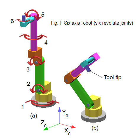
In the first tutorial we introduced the six axis robot shown in Fig.1 above, which is our model for kinematic analysis. Each link is shaded a different colour. We use the physical construction of the robot to draw a kinematic diagram which defines the co-ordinate system (called a frame) for each joint.

Firstly we define co-ordinates for the base or "real world" frame, shown on Fig.1*. This co-ordinate frame is indicated by subscript 0. Its origin is at the centre of the top surface of the base plate (shaded grey). This is a "right hand" co-ordinate system (check images on-line if you are not familiar with the right-hand rule). In the right hand rule counter-clockwise rotation about an axis is designated +ve.

*The co-ordinates shown are those of the CAD model I used as the basis of this tutorial. It is more conventional for Z to be the vertical co-ordinate in the base frame.

Each joint is assigned a co-ordinate frame located at some point on its axis of rotation. Co-ordinate frames form the basis of the kinematic diagram and the first task is to fix their position.

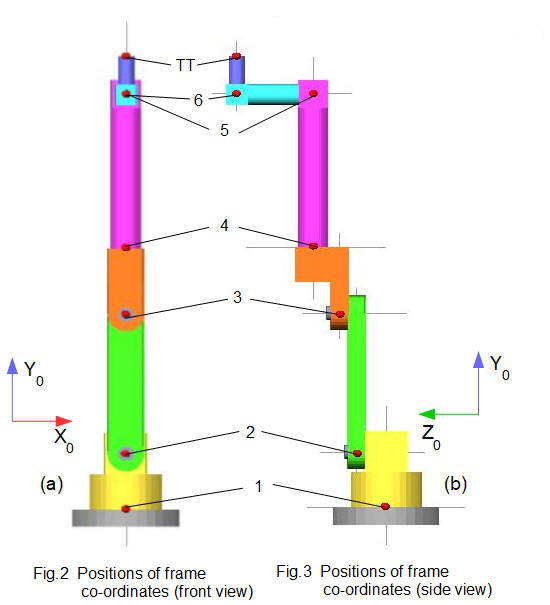
Figs.2 and 3 below show the construction of the robot model in a vertically extended pose with front view on the XY plane, and side view on the YZ plane. Red dots show the chosen location of each frame for joints #1 to #6. The tool tip at the end face of the final link has the frame designated TT. The frame for joint 1 is coincident with the base frame.

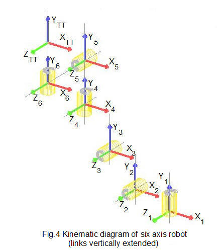
The first stage of the kinematic diagram is shown in Fig.4 below with co-ordinate frames in three dimensions for each joint in the vertically extended pose. Revolute joints are represented by cylinders. For clarity the diagram is not drawn to scale . In this pose, orientations of X, Y and Z axes in each frame are chosen to be identical but this is not essential. The origin of a frame can be at any convenient point on the axis of joint rotation and can even be outside the physical joint (as we shall see in the next tutorial).

We now add to the diagram the length and offset of each link. The link length is the distance between successive frames on the longitudinal axis of the link,not the external dimension of the link. An offset occurs where the co-ordinate frames of two linked joints do not lie on the same axis. In this pose the robot model has offsets on the Z axis only.

Fig.5 below shows link lengths and offsets on the kinematic diagram viewed on the YZ plane which provides a clearer view than the three dimensional diagram in Fig.4. Again note that this diagram is not to scale. Link lengths are denoted by a single subscript and offsets by a twin subscript, for example a₁ is the link length between joint #1 and joint #2 and a₁₂ is the offset between these joints.

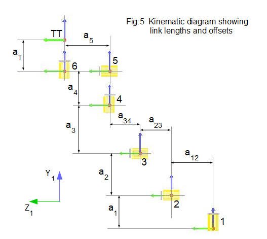
The table below lists dimensions of links and offsets in the robot model (unspecified length units).

Finally, we require the angle of rotation applied to each joint to achieve the tool tip pose shown in Fig.1(b). In this example the joint rotations are:

• joint #2   rotate 45° counter-clockwise


• joint #3   rotate 90° clockwise


• joint #5   rotate 90° clockwise

The next section explains how we express movement of the robot mathematically using transformations of co-ordinate frames.

Rotation and translation of co-ordinate frames

The objective of forward kinematic analysis is to compute the real world co-ordinates of the tool tip with reference to the base frame. When a revolute joint rotates, its co-ordinate frame rotates about the joint axis. Also we must take account of displacements between frames denoted by link lengths and offsets, where the latter exist. Hence we need a method for resolving displacements in three dimensions that result from rotation of the joints, beginning at the base frame and finishing at the tool tip.

The most widely applied method which we outline below uses transformation matrices to combine rotation and translation of co-ordinate frames (translation simply means linear displacement). The following derivation of transformation matrices is presented in terms of vector transformations. The first part concerns rotation and the second part translation.

Rotation of co-ordinate frames

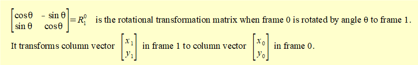
Figs.6 (a) and (b) show rotation of a right hand co-ordinate frame* about the Z axis. We consider initially this rotation in two dimensions in the XY plane.

*It is conventional to use the notation X₀, Y₀, Z₀. for the base frame.

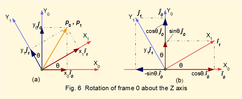
(in the following text vectors are indicated in bold italic type)

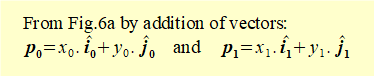
Co-ordinate frame 0 with axes X₀ and Y₀ is rotated counter-clockwise by angle θ to create a second frame 1 with axes X₁ and Y₁. We envisage the axis of rotation coming out of the XY plane indicated by the green dot.

i₀,  j₀,  i₁ and j₁ are unit vectors on the X₀, Y₀, and X₁ Y₁ axes respectively and are represented by the lengths of the axis arrows

Fig 6a shows a position vector p₀ for a point p in space with co-ordinates x₀ and y₀ in frame 0. The position vector for point p referred to rotated frame 1 is p₁ with co-ordinates x₁ and y₁. Note that p₀ ≠ p₁*.

*p₀ ≠ p₁ because these vectors are in frames of reference that are not parallel. However, the relationships developed below based on the geometrical configuration are valid.

Substituting the above expressions for i₁ and j₁ into the above expression for p₁ gives:

We can state these equations in matrix form as:

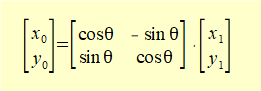
Examining the columns of the matrix we see that columns 1 and 2 are respectively column vectors for: (i) the projections of X₁ on X₀ and Y₀ and (ii) the projections of Y₁ on X₀ and Y₀, where X₁ and Y₁ have the magnitude of unit vectors i₁ and j₁.

We now expand the rotational matrix to three dimensions by introducing axes Z₀ and Z₁ and adding projections of X₁ and Y₁ on Z₀ and projections of Z₁ on X₀, Y₀ and Z₀.

In Figs.6a and 6b the Z axis is perpendicular out of the page hence projections of X₁ and Y₁ on Z₀ = 0 and projections of Z₁ on X₀ and Y₀ = 0. The projection of Z₁ on Z₀ = 1 since the Z axis is unchanged by the rotation. We can now expand the transformation matrix for rotation about the Z axis from two to three dimensions as follows:

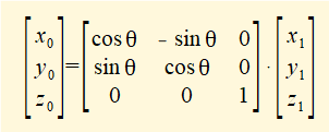
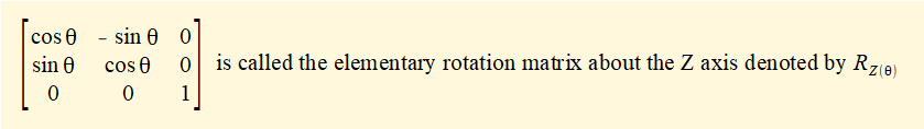
The notation R_Z(θ) indicates a rotation matrix for a rotation angle θ about the Z axis.

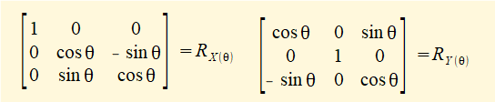
The corresponding elementary rotation matrices R_X(θ) and R_Y(θ) for rotation about the X and Y axes respectively are:

Rotation matrices can be multiplied by dot product to obtain a transformation matrix for a series of frame rotations. Thus if the rotation of frame 0 to frame 1 about axis Z₀ is angle θ and the rotation of frame 1 to frame 2 about axis Z₁ is angle φ then:

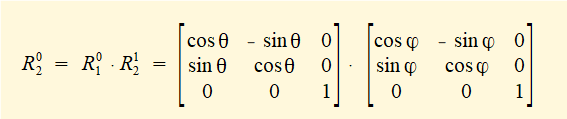
The reverse rotational transformation matrix from frame 0 to frame 1 is the transpose of R⁰₁
i.e.  R¹₀ = (R⁰₁,)T

It seems illogical to apply backward frame transformations in forward kinematics. This makes sense however because as we move angular positions of each link progressively forward to the tool tip we transform the frame co-ordinates of the forward positions back to the real world co-ordinates of the first frame.

Translation of co-ordinate frames

By translation we mean moving the origin of a co-ordinate frame to a new point in space. In the context of forward kinematics the new point is the origin of the co-ordinate frame for the next joint.

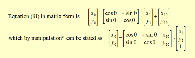
It is useful to combine translation and rotation in one transformation matrix. We now show how this is done, initially in two dimensions and then expanded to three dimensions.

Figs.7a and 7b below show co-ordinate frame 1 rotated and then translated in the XY plane from its original position coincident with frame 0.

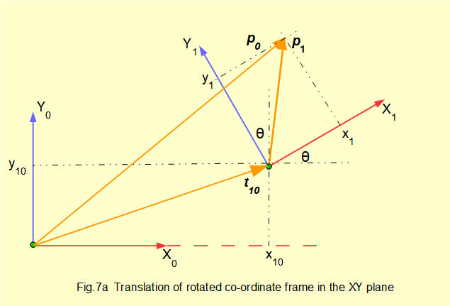
In Fig 7a consider point p in space represented by position vector p₁ in frame 1 with co-ordinates x₁ and y₁. Point p is also represented by position vector p₀ in frame 0. However, vectors p₁ and p₀ cannot be added legitimately because co-ordinate frames 0 and 1 are not parallel. Vector t₁₀ is the position vector of the origin of frame 1 in frame 0.

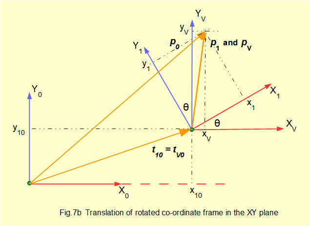
In Fig 7b we introduce a co-ordinate frame V which is parallel to frame 0 and shares its origin with frame 1. Point p is now represented by position vector p_v in frame V. Note that p_v ≠ p₁ . The origin of frame V with respect to frame 0 is represented by vector t_v0 which is equal to vector t₁₀

Because frame V is parallel to frame 0 we can add vectors in frames 0 and V such that:

p₀ = t_v0 + p_v ................ (i)

Now we replicate frame 1 by rotating frame V by angle θ, using rotational transformation matrix R^v₁

which gives :   p_v = R^v₁ . p₁ ................... (ii)

substituting for p_v in (i) gives:   p₀ = t_v0 + R^v₁ . p₁

now:   R^v₁ = R⁰₁ (equal rotations of angle θ) and t_v0 = t₁₀

giving:   p₀ = t₁₀ + R^v₁ . p₁ ..................... (iii)

*this step is not obvious but is easily checked by expanding dot products in both equations.

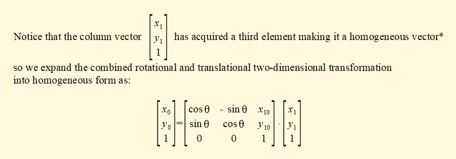
*Homogeneous co-ordinates add one dimension to Cartesian co-ordinates and are widely used for linear transformations in computing

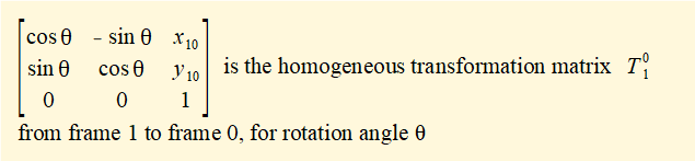
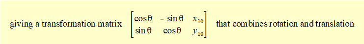
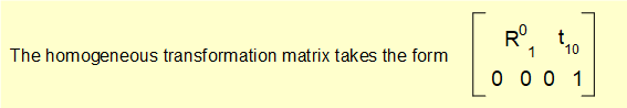
Note that the homogeneous transformation matrix takes the form:

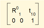
where R⁰₁ is the rotational transformation matrix and t₁₀ is the column vector representing translation of the origin of frame 1 to the origin of frame 0.

The reverse homogeneous transformation matrix for a transformation from frame 0 to frame 1 is the inverse of T⁰₁, i.e. where T¹₀ = (T⁰₁)^-1 (not the transpose as for the reverse transformation of R⁰₁)

Homogeneous transformation matrices can be multiplied to obtain a transformation matrix for a series of frame rotations and translations such that T⁰₂ = T⁰₁ . T¹₂

Derivation of the homogeneous transformation matrix for three dimensions is broadly identical to the two dimensional case using homogeneous vectors with X, Y and Z components. The result is a [4 x 4] homogeneous transformation for rotation about the Z axis as follows.

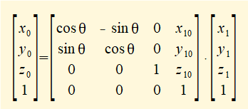
Where R⁰₁ is the elementary rotation matrix and t₁₀ is the column vector representing translation of the origin of co-ordinate frame 0 to the origin of co-ordinate frame 1. We call the vector t₁₀ the translation (or displacement) vector.

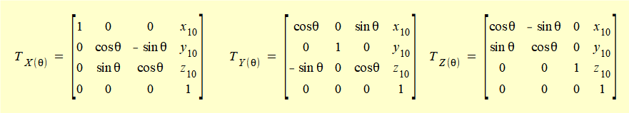
The homogeneous transformation matrices for rotation about the X, Y and Z axes are thus:

As with the two dimensional case we can combine homogeneous transformations to obtain a transformation matrix for a series of frame rotations and translations such that:

T⁰_n = T⁰₁ • T¹₂ • ----- •T^(n-1)_n.

Examination of the dot product shows that the translation vector part t_n0 of matrix T⁰_n expresses the co-ordinates of the origin of frame n with respect to frame 0.

We now have a mathematical tool for forward kinematic analysis of the robot model. The next section of the tutorial examines each joint of the robot in forward sequence, applying the homogeneous transformation matrix at each stage.

Frame by frame analysis of the robot model

Commercial software for applications in robotics (for example MATLAB) computes multiple matrix transformations using joint angles, link lengths and offsets as input variables. For our purpose, however, it is instructive to compute each transformation in forward kinematics using an online matrix calculator to find the real world co-ordinates of each joint. All frame co-ordinates derived below have been validated directly from the CAD robot model.

As a starting point it is useful to view the robot model from Fig 1 showing the vertical datum pose and the specified operating pose.

To suit the CAD model I choose the datum position for the robot with links in vertical extension on the Y axis, however note that it is equally valid to begin with horizontal extension of links on the X axis.

Also note that signs for angles of rotation θ (counter-clockwise positive, clockwise negative) apply only to the rotation section of the homogeneous transformation matrix. Signs for displacements in the translational column vector section are in accordance with the applicable frame axes

Transformation - frame 1 to frame 0

We recall in this model that the co-ordinates of frame 0 are the real world co-ordinates of the static base plate (grey colour). Also that the origin of frame 1 for joint 1 is co-incident with frame 0.

In the specified pose joint 1 has no rotation, thus the homogeneous* transformation matrix from frame 1 to frame 0 is the identity matrix (θ = 0) which we omit from succeeding matrix dot product chains. In this instance the origin of frame 1 is a proxy for the origin of real world co-ordinates.

*from this point in the text the term transformation matrix refers to the homogeneous version.

Transformation - frame 2 to frame 1

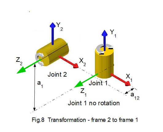
Fig.8 is an enlarged section of the kinematic diagram in Fig.3 showing the orientation of frame 2 translated from frame 1 without rotation of frame 1. The initial state of frame 1 has real world co-ordinates x₁ = 0, y₁ = 0, z₁ = 0 (i.e. identical to the co-ordinates of the base frame).

Parameters for transformation T¹₂ are:

• there is no rotation of frame 1. Thus θ₁ = 0°


• frame 2 translates to frame 1 along link length a₁ on the Y axis and link offset a₁₂ on the Z axis.


• link length a₁ = 160


• link offset a₁₂ = 85

Inserting these values into the homogeneous transformation matrix for rotation about the Y axis gives:

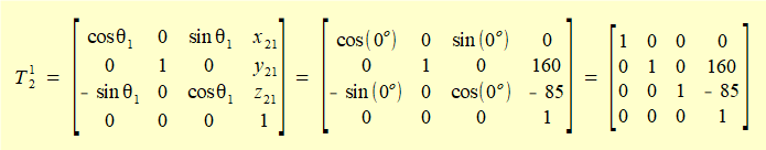
Note that the rotational part of the transformation matrix in the upper left hand section is the identity matrix. This is consistent with no rotation.

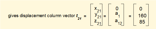
We use the transformation matrix T¹₂ to state co-ordinates x₂, y₂, z₂ within frame 2 in terms of co-ordinates x₁, y₁, z₁ within frame 1 from the equation:

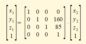
The origin of frame 2 has co-ordinates: x₂ = 0, y₂ = 0, z₂ = 0 giving:

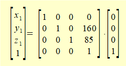
Note that the translation vector t₂₁ in the transformation matrix yields the required real world co-ordinates. This result was predictable since frame 2 does not rotate relative to the base. Examining the above dot product reveals that the translation vector t_n1 in every transformation matrix T¹_n yields the real world co-ordinates in frame 1 of the origin of each frame n.

We now progress through the remaining transformations with the objective of determining the translation vector in each transformation matrix.

Transformation - frame 3 to frame 2

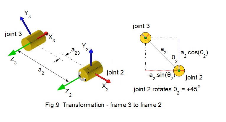
Fig.9 shows the orientation of frame 3 translated from frame 2 with joint 2 rotated through angle θ₂.

Projections of link length a₂ are a₂.cosθ₂ on the Y axis and - a₂.sinθ₂ on the X axis.

Parameters for transformation T²₃ are:

• frame 2 rotates 45° on the Z axis in a positive (counter-clockwise) direction. Thus θ₂ = 45°


• frame 2 translates to frame 3 along link length a₂ and link offset a₂₃ on the Z axis.


• link length a₂ = 400


• link offset a₂₃ = 50

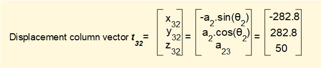
Inserting these values into the transformation matrix for rotation about the Z axis gives:

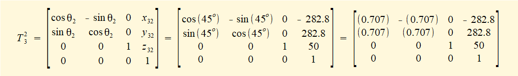
Now perform the matrix multiplication T¹₃ = T¹₂ • T²₃ giving:

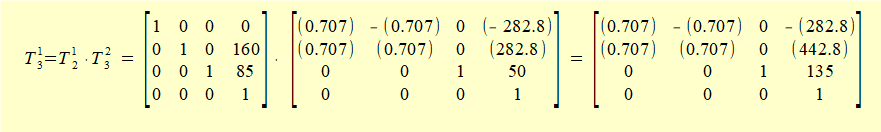
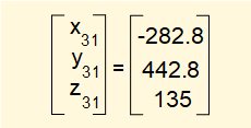
Hence real world co-ordinates of the origin of frame 3 after rotation of joint 2 read from the t₃₁ section of matrix T¹₃ are:

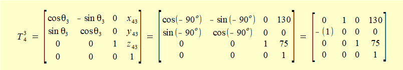
Transformation - frame 4 to frame 3

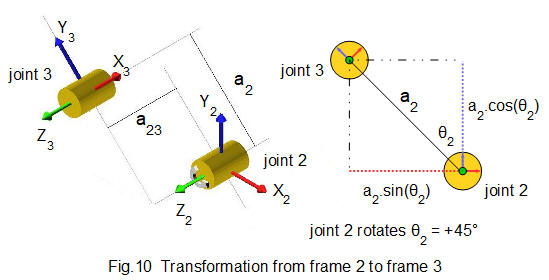
Fig.10 shows the orientation of frame 4 translated from frame 3 with joint 3 rotated through angle θ₃ (for clearer illustration the viewpoint of Fig.10 has changed from previous diagrams).

Projections of link length a₃ are a₃.cosθ₃ = 0 on the Y axis and a₃.sinθ₃ = a₃ on the X axis.

Parameters for transformation T³₄ are:

• frame 3 rotates 90° around the Z axis in a negative (clockwise) direction. Thus θ₃ = -90°


• frame 3 translates to frame 4 along link length a₃ and link offset a₃₄ on the Z axis.


• link length a₃ = 130


• link offset a₃₄ = 75

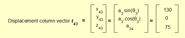
Inserting these values into the transformation matrix for rotation about the Z axis gives:

Now perform the matrix multiplication T¹₄ = T¹₃ • T³₄ giving:

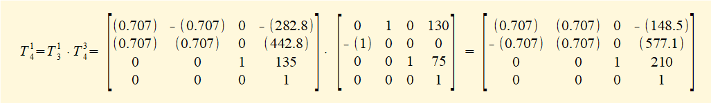
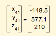
Hence real world co-ordinates for the origin of frame 4 after the transformation read from the t₄₁ section of matrix T¹₄ are as follows:

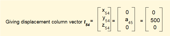
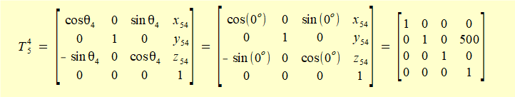
Transformation - frame 5 to frame 4

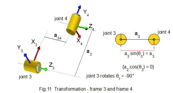
Fig.11 shows the orientation of frame 5 translated from frame 4 without rotation of joint 4.

Parameters for transformation T⁴₅ are:

• there is no rotation: thus θ₄ = 0°


• frame 4 translates to frame 5 along link length a₄. There is no link offset on the Z axis.


• ink length a₄= 500

Inserting these values into the transformation matrix for rotation about the Y axis gives:

Now perform the matrix multiplication T¹₅ = T¹₄ • T⁴₅ giving:

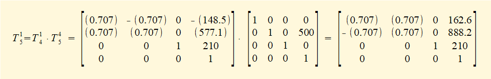
Hence real world co-ordinates for the origin of frame 5 after the transformation read from the t₅₁ section of matrix T¹₅ are as follows:

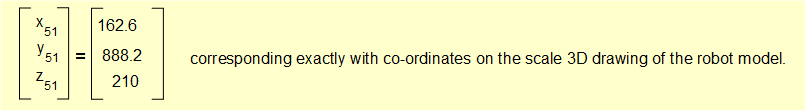
Transformation - frame 6 to frame 5

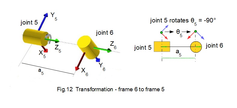
Fig.12 shows the orientation of frame 6 translated from frame 5 with joint 5 rotated through angle θ₅.

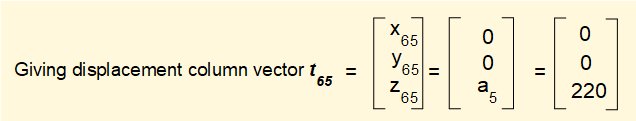
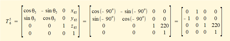
Parameters for transformation T⁵₆ are:

• frame 5 rotates 90° in a negative (clockwise) direction about the Z axis. Thus θ₅ = -90°


• frame 5 translates to frame 6 along link length a₅ on the Z axis.


• link length a₅ = 220

Inserting these values into the transformation matrix for rotation about the Z axis gives:

Now perform the matrix multiplication T¹₆ = T¹₅ • T⁵₆ giving:

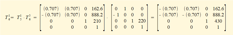
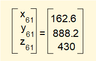
Hence real world co-ordinates for the origin of frame 6 after the transformation read from the t₆₁ section of matrix T¹₆ are as follows:

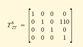
Transformation - frame TT (tool tip) to frame 6

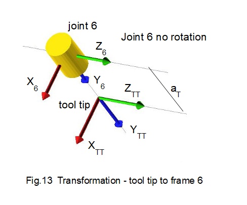
Fig.13 shows the orientation of the tool tip frame translated from frame 6 without rotation of joint 6.

Parameters for transformation T⁶_TT are:

• there is no rotation. Thus θ₆ = 0°


• frame 6 translates to frame TT along link length a_T on the Y axis


• link length a_T = 110

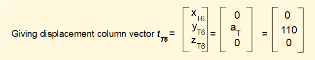
No rotation is equivalent to placing the identity matrix in the rotation section of the transformation matrix Thus T⁶_TT can be stated as:

Now perform the matrix multiplication T¹_TT = T¹₆ • T⁶_TT giving:

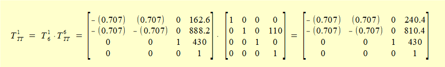
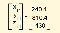
Hence real world co-ordinates for the origin of frame TT after the transformation read from the t_TT1 section of matrix T¹_TT are as follows:

We have completed the forward kinematic analysis using homogeneous transformations. In the next tutorial we demonstrate another method of forward analysis using transformation matrices known as the Denavit Hartenberg method.

Next:  Kinematics of robot manipulators - forward kinematics 2

return to home page

I welcome feedback at:

alistair@alistairstutorials.co.uk