If you are unfamiliar with basic principles of robot manipulators I suggest reading the introduction to this series.
This tutorial continues from the previous tutorial which covers forward kinematic analysis using homogeneous transformation matrices. We now examine the Denavit Hartenberg (DH) method using a modified homogeneous transformation matrix to find the real world co-ordinates of the tool tip where the joint angles are given. The advantage of the DH method is that only four parameters are required to define transformations, as opposed to six for the previous method (three rotations and three translations). Four input parameters are more economical than six in computing software terms. It is fair to say however that the DH method is more complex using manual calculations.
Firstly we explain the DH method and then work through the transformation stages using our robot model as an example.
Rules for applying the DH method
Rules for co-ordinate frames
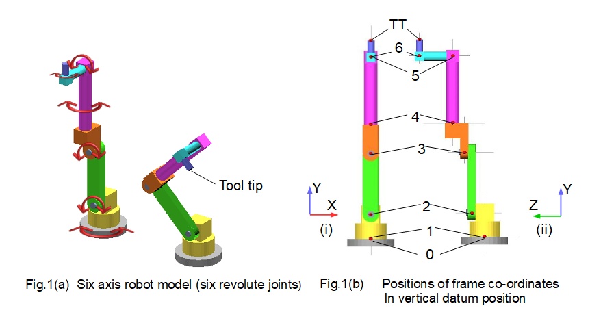
Fig.1 above shows the six axis robot model used in the previous tutorial, illustrating the vertical datum position and the tool tip pose produced by specified joint angles. Frame 0, coincident with the origin of frame 1, represents the real world co-ordinates of the base frame (grey colour).
The DH method requires co-ordinate frames set up in accordance with very specific rules which we now state. Co-ordinate frames are considered in pairs, successive frames being designated frame n and frame (n-1) with co-ordinates denoted Xn, X(n-1), etc.
Rule 1: The axis of rotation of every frame associated with a revolute joint must be the Z axis (also applies to the axis of linear movement for a prismatic joint).
Rule 2: Axis Xn must be perpendicular to axis Z(n-1)
Rule 3: Axis Xn must intersect axis Z(n-1) . To achieve this requirement frame n can: (a) be rotated, or (b) translated along one of the joint axes.
Rule 4: The Y axis in all frames must be orientated in accordance with the right hand rule.
Setting up co-ordinate frames
We now set up each pair of co-ordinate frames in the robot model in accordance with DH rules. Diagrams and summaries explain the process.
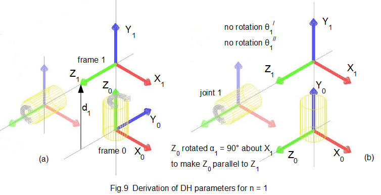
Frame 1
Fig.2 below illustrates DH rules for frame co-ordinates applied to frame 1 associated with joint 1. Note that DH rules do not apply to frame 0 as the static base frame is not a joint. It follows that rules 2 and 3 relating to the (n-1) joint do not apply in this case. The origin of frame 1 is coincident with the origin of frame 0 which represents the origin of real world co-ordinates
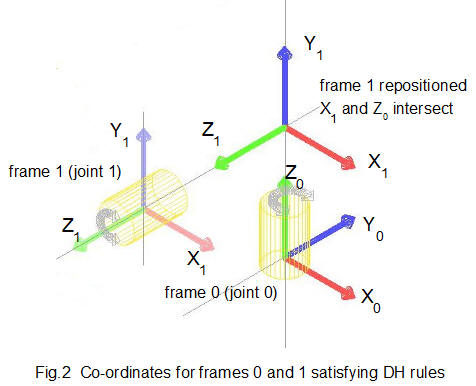
- Z axis is the axis of rotation.
- Y axis corresponds to the right-hand rule
Frame 2
Fig.3 below illustrates DH rules for frame co-ordinates applied to frame 2 (associated with joint 2). In this case frame 2 is frame n and frame 1 is frame (n-1)
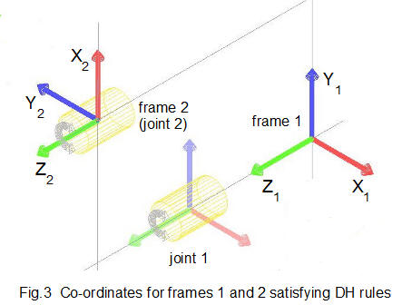
- Z2 is the axis of joint rotation
- Axis X2 is perpendicular to axis Z1
- In its original position at the centre of joint 2 axis X2 does not intersect axis Z1. By moving frame 2 along the Z2 axis we obtain the necessary intersection shown in Fig.3.
- Y2 axis corresponds to the right-hand rule
Frame 3
Fig.4 below illustrates DH rules for frame co-ordinates applied to frame 3 (associated with joint 3). In this case frame 3 is frame n and frame 2 is frame (n-1)
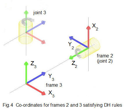
- Z3 is the axis of joint rotation
- Axis X3 is perpendicular to axis Z2
- Axis X3 intersects axis Z2
- Y axis corresponds to the right-hand rule
Frame 4
Fig.5 below illustrates DH rules for frame co-ordinates applied to frame 4 (associated with joint 4). In this case frame 4 is frame n and frame 3 is frame (n-1)
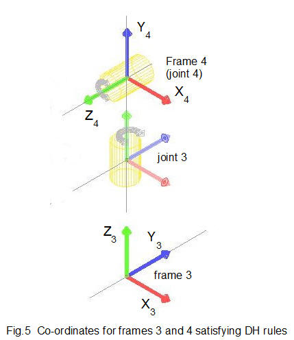
- Z4 is the axis of joint rotation
- In its original position at the centre of joint 4 axis X4 does not intersect axis Z3. By moving frame 4 along the Z4 axis we obtain the necessary intersection shown in Fig.5.
- Axis X4 is perpendicular to axis Z3
Frame 5
Fig.6 below illustrates DH rules for frame co-ordinates applied to frame 5 (associated with joint 5). In this case frame 5 is frame n and frame 4 is frame (n-1)
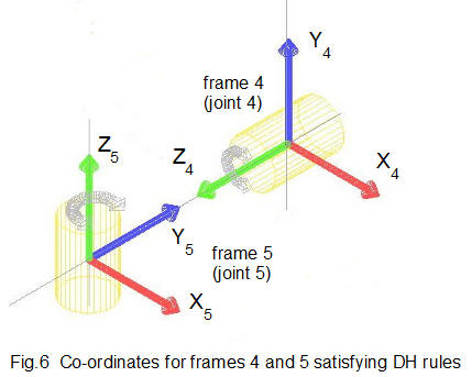
- Z5 is the axis of joint rotation
- Axis X5 is perpendicular to axis Z4
- Axis X5 intersects axis Z4
- Y axis corresponds to the right-hand rule
Frame 6
Fig.7 below illustrates DH rules for frame co-ordinates applied to frame 6 (associated with joint 6). In this case frame 6 is frame n and frame 5 is frame (n-1)
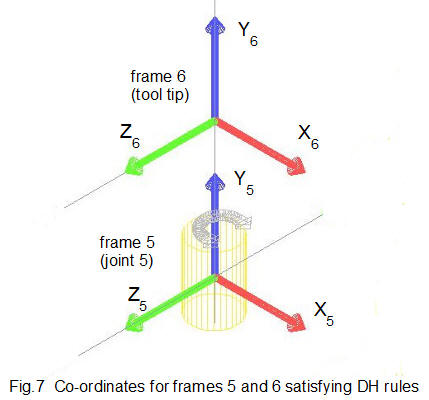
- Z6 is the axis of joint rotation
- Axis X6 is perpendicular to axis Z5
- Axis X6 intersects axis Z5
- Y axis corresponds to the right-hand rule
Frame TT (tool tip)
Fig.8 below illustrates frame co-ordinates applied to the tool tip. Because the tool tip is not a joint the DH rules do not apply. We compute the transformation from the tool tip to frame 6 using the standard homogeneous transformation matrix T6TT where the rotational part of the matrix is the identity matrix because there can be no relative rotation between the tool tip and frame 6.
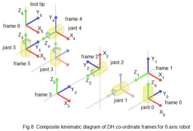
Fig. 9 below shows the complete set of co-ordinate frames for forward kinematic analysis of this six axis robot using the DH method.
Definition of DH parameters
With the co-ordinate frames set up according to DH rules we now define the four DH parameters designated θ, α (alpha), r * and d.
* sometimes denoted by a but easily mistaken in print for α
Parameter θ
θn is the addition of two angles:
- angle 1 is the angle required to rotate axis X(n-1) around axis Z(n-1) such that axis X(n-1) is parallel to axis Xn. We will denote angle 1 as θ/n
- angle 2 is the angle the revolute joint associated with frame (n-1) rotates around axis Z(n-1). We will denote angle 2 as θ//n
Parameter α
αn is the angle required to rotate axis Z(n-1) around axis Xn such that axis Z(n-1) is parallel to axis Zn
Parameter r
rn is the displacement in the Xn direction from the centre of frame (n -1) to the centre of frame n .
Parameter d
dn is the displacement in the Z(n-1) direction from the centre of frame (n -1) to the centre of frame n .
These parameters will become clearer as we work through each pair of co-ordinate frames. Note that rotations around and displacements along the Y axis play no active part in the DH method.
DH parameters are normally presented in a table shown below with each co-ordinate pair designated by a number n. Our robot model has 6 co-ordinate pairs giving the following parameter table.
| Frames | n | θ | α | r | d |
|---|---|---|---|---|---|
| 1, 2 | 2 | ||||
| 2, 3 | 3 | ||||
| 3, 4 | 4 | ||||
| 4, 5 | 5 | ||||
| 5, 6 | 6 |
DH homogeneous transformation matrix
In the previous tutorial we derived homogeneous transformation matrices, T combining:
- rotation angle θ of co-ordinate frame X0, ,Y0 , Z0 about axis X0, ,Y0 ,or Z0 to create a new frame X1 ,Y1 ,Z1
- translation of the origin of frame X0, Y0, Z0 to a position defined by vector [x10, y10, z10].
For rotation about X, Y and Z axes respectively the transformation matrices are:
The DH transformation matrix is the combination of two rotations and two displacements for designated axes in the DH co-ordinate frames.
Examining the criteria for DH parameters it is seen that the applicable rotation axes are:
- Z(n-1) for which the parameter is θn
- Xn for which the parameter is αn
The applicable displacement axes are:
- Z(n-1) for which the parameter is dn
- Xn for which the parameter is rn
The DH transformation matrix T(n-1)n is a serial combination of homogeneous transformation matrices as follows.
T(n-1)n = Dd • Rθ • Dr • Rα where:
- D denotes a transformation matrix for displacement where the rotation part of the matrix is the identity matrix.
- R denotes a transformation matrix for rotation where the displacement part of the matrix is the zero vector.
Giving:
Frame by frame computation
We now compute the DH matrix for each paired set of frames n and (n-1). In each case the first task is to determine values of θn, αn , rn and dn using the physical parameters of the robot model noting that joint rotations producing the specified tool tip pose are as follows:
| joint # | rotation angle |
|---|---|
| 1 | 0° |
| 2 | 45° |
| 3 | -90° |
| 4 | 0° |
| 5 | -90° |
| 6 | 0° |
Pair 1 - frame 1 and frame 2 (n = 2)
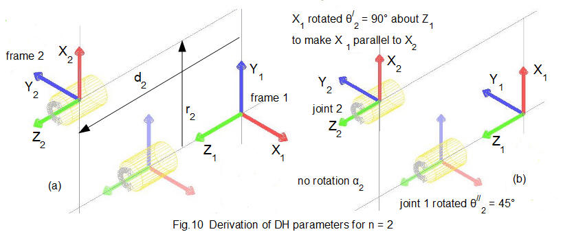
Fig.10(a) above shows frame 1 and frame 2 set up using the DH rules as shown in Figs.2 and 3. Frame 2 is frame n and frame 1 is frame (n-1.) Consider each DH parameter in turn. Fig.10(b) shows the orientation of frames 1 after rotations θ/1 and α1.
Parameter θ1
θ/1 is the angle required to rotate axis X1 around axis Z1 such that axis X1 is parallel to axis X2. Fig.9(a) shows X1 is already parallel to X2. Thus θ/1 = 0°.
θ//1 is the angle revolute joint 1 rotates around axis Z1. In this case θ//1 = 0°.
Thus: θ1 = θ/1 + θ//1 = 0°
Parameter α1
α1 is the angle required to rotate axis Z1 around axis X2 such that axis Z1 is parallel to axis Z2 . Fig.10 shows Z1 must be rotated 90° counter-clockwise around X2 for Z1 to be parallel to Z2. Thus α1 = 90°.
Parameter r1
r1 is the displacement in the X2 direction from the centre of frame 1 to the centre of frame 2. Fig10 shows there is no displacement between the frame centres in the X2 direction. Thus r1 = 0.
Parameter d1
d1 is the displacement in the Z1 direction from the centre of frame 1 to the centre of frame 2 as shown on Fig.10. From the robot model d1 = 160 *.
* We use unspecified units of length for displacements
The first row of the DH parameter table is now complete.
| Frames | n | θ | α | r | d |
|---|---|---|---|---|---|
| 1, 2 | 2 | 0° | 90° | 0 | 160 |
We compute the DH transformation matrix T12 to give:
* Recall from above that the origin of frame 1 is coincident with the origin of the base frame co-ordinates and thus represents real world co-ordinates. Also note that the real world co-ordinates of frame 2 are not the real world co-ordinates of the centre of joint 2 because frame 2 was translated along the Z2 axis to satisfy DH rule 3 for setting up frame co-ordinates.
Pair 2 - frame 2 and frame 3 (n = 3)
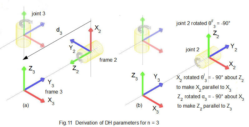
Fig.11(a) above shows frame 2 and frame 3 set up using the DH rules as shown in Figs.3 and 4. Frame 3 is frame n and frame 2 is frame (n-1.) Consider each DH parameter in turn. Fig.11(b) shows the orientation of frames 2 after rotations θ/2 and α2.
Parameter θ2
θ/2 is the angle required to rotate axis X2 around axis Z2 such that axis X2 is parallel to axis X3 . Fig.11 shows X2 must be rotated 90° counter-clockwise around Z2 to be parallel to X3. Thus θ/2 = 90°.
θ//2 is the angle revolute joint 2 rotates around axis Z2 . In this example θ//2 = 45°.
Thus: θ2 = θ/2 + θ//2 = 90° + 45° = 135°
Parameter α2
α2 is the angle required to rotate axis Z2 around axis X3 such that axis Z2 is parallel to axis Z3 . Fig.11 shows Z2 is already parallel to Z3. Thus α2 = 0°.
Parameter r2
r2 is the displacement in the X3 direction from the centre of frame 2 to the centre of frame 3 as shown on Fig.11. From the robot model, r2 = 400.
Parameter d2
d2 is the displacement in the Z2 direction from the centre of frame 2 to the centre of frame 3 as shown on Fig11. From the robot model d2 = 135.
The second row of the DH parameter table is now complete.
| Frames | n | θ | α | r | d |
|---|---|---|---|---|---|
| 1, 2 | 2 | 0° | 90° | 0 | 160 |
| 2, 3 | 3 | 135° | 0° | 400 | 135 |
We compute the DH transformation matrix T23 to give* :
Pair 3 - frame 3 and frame 4 (n = 4)
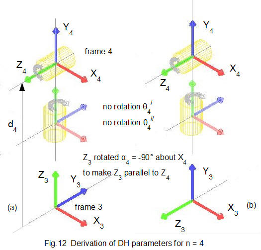
Fig.12(a) above shows frame 3 and frame 4 set up using the DH rules as shown in Figs.3 and 4. Frame 4 is frame n and frame 3 is frame (n-1.) Consider each DH parameter in turn. Fig.12(b) shows the orientation of frames 3 after rotations θ/3 and α3.
Parameter θ3
θ/3 is the angle required to rotate axis X3 around axis Z3 such that axis X3 is parallel to axis X4. Fig.12 shows X3 must be rotated 90° clockwise around Z3 to be parallel to X4. Thus θ/3 = -90°.
θ//3 is the angle revolute joint 3 rotates around axis Z3. In this example θ//3 = -90°.
Thus: θ3 = θ/3 + θ//3 = -90° + (-90°) = -180°
Parameter α3
α3 is the angle required to rotate axis Z3 around axis X4 such that axis Z3 is parallel to axis Z4 . Fig.12 shows Z3 must be rotated 90° clockwise around X4 to be parallel to Z4. Thus α3 = -90°.
Parameter r3
r3 is the displacement in the X3 direction from the centre of frame 3 to the centre of frame 4 as shown on Fig.12. In this case r3 = 0.
Parameter d3
d3 is the displacement in the Z3 direction from the centre of frame 3 to the centre of frame 4 as shown on Fig12. From the robot model, d3 = 75.
The third row of the DH parameter table is now complete.
| Frames | n | θ | α | r | d |
|---|---|---|---|---|---|
| 1, 2 | 2 | 0° | 90° | 0 | 160 |
| 2, 3 | 3 | 135° | 0° | 400 | 135 |
| 3, 4 | 4 | -180° | -90° | 0 | 75 |
We compute the DH transformation matrix T34 to give:
and then compute T14 = T13 • T3 4 giving:
Pair 4 - frame 4 and frame 5 (n = 5)
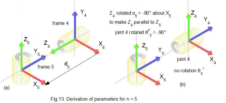
Fig.13(a) above shows frame 4 and frame 5 set up using the DH rules as shown in Figs.3 and 4. Frame 5 is frame n and frame 4 is frame (n-1.) Consider each DH parameter in turn. Fig.13(b) shows the orientation of frames 4 after rotations θ/4 and α4.
Parameter θ4
θ/4 is the angle required to rotate axis X4 around axis Z4 such that axis X4 is parallel to axis X5 . Fig.13 shows X4 is already parallel to X5. Thus θ/4 = 0°.
θ//4 is the angle revolute joint 4 rotates around axis Z4. In this example θ//4 = 0°.
Thus: θ4 = θ/4 + θ//4 = 0° + 0° = 0°
Parameter α4
α4 is the angle required to rotate axis Z4 around axis X5 such that axis Z4 is parallel to axis Z5. Fig.13 shows Z4 must be rotated 90° counter-clockwise around X5 to be parallel to Z5. Thus α4 = 90°.
Parameter r4
r4 is the displacement in the X4 direction from the centre of frame 4 to the centre of frame 5 as shown on Fig.13. In this case r4 = 0.
Parameter d4
d4 is the displacement in the Z4 direction from the centre of frame 4 to the centre of frame 5 as shown on Fig.13. From the robot model, d4 = 630.
The fourth row of the DH parameter table is now complete.
| Frames | n | θ | α | r | d |
|---|---|---|---|---|---|
| 1, 2 | 2 | 0° | 90° | 0 | 160 |
| 2, 3 | 3 | 135° | 0° | 400 | 135 |
| 3, 4 | 4 | -180° | -90° | 0 | 75 |
| 4, 5 | 5 | 0° | 90° | 0 | 630 |
We compute the DH transformation matrix T45 to give:
and then compute T15 = T14 • T4 5 giving:
Pair 5 - frame 5 and frame 6 (n = 6)
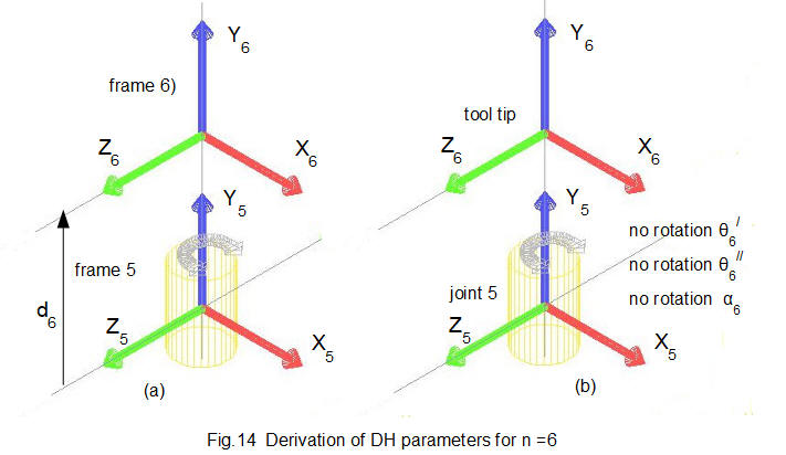
Fig.14(a) above shows frame 5 and frame 6 set up using the DH rules as shown in Figs.3 and 4. Frame 6 is frame n and frame 5 is frame (n-1.) Consider each DH parameter in turn. Fig.14(b) shows the orientation of frames 5 after rotations θ/5 and α5.
Parameter θ5
θ/5 is the angle required to rotate axis X5 around axis Z5 such that axis X5 is parallel to axis X6 . Fig.14 shows X5 is already parallel to X6. Thus θ/5 = 0°.
θ//5 is the angle revolute joint 5 rotates around axis Z5. In this example θ//5 = -90°.
Thus: θ5 = θ/5 + θ//5 = 0° + (-90°) = -90°
Parameter α5
α5 is the angle required to rotate axis Z5 around axis X6 such that axis Z5 is parallel to axis Z6. Fig.14 shows Z5 must be rotated 90° clockwise around X6 to be parallel to Z6. Thus α5 = -90°.
Parameter r5
r5 is the displacement in the X5 direction from the centre of frame 5 to the centre of frame 6 as shown on Fig.14. In this case r5 = 0.
Parameter d5
d5 is the displacement in the Z5 direction from the centre of frame 5 to the centre of frame 6 as shown on Fig.14. From the robot model, d5 = 220.
The fifth row of the DH parameter table is now complete.
| Frames | n | θ | α | r | d |
|---|---|---|---|---|---|
| 1, 2 | 2 | 0° | 90° | 0 | 160 |
| 2, 3 | 3 | 135° | 0° | 400 | 135 |
| 3, 4 | 4 | -180° | -90° | 0 | 75 |
| 4, 5 | 5 | 0° | 90° | 0 | 630 |
| 5, 6 | 6 | -90° | -90° | 0 | 220 |
We compute the DH transformation matrix T56 to give:
and then compute T16 = T15 • T5 6 giving:
Transformation from tool tip to frame 6
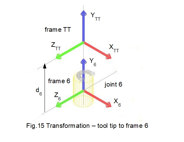
Fig.15 shows co-ordinates for frame 6, associated with revolute joint 6, and the tool tip as established in Fig.8.
As stated previously we compute the transformation from the tool tip to frame 6 using the standard homogeneous transformation matrix T6TT where the rotational part of this matrix is the identity matrix since there can be no relative rotation between frame 6 and the tool tip.
Thus T6TT can be stated as:
Now perform the matrix multiplication T1TT = T16 • T6TT giving:
And the marathon Denavit Hartenberg forward kinematic analysis is complete!
Note that the real world co-ordinate system used in this tutorial differs from the one used in the previous tutorial. Both are right handed co-ordinate systems but Y and Z axes are interchanged with the sign reversing in the change from Z axis to Y axis.
Next: Kinematics of robot manipulators - inverse kinematics
I welcome feedback at: