In the previous two tutorials we examined methods of forward kinematics for a six axis robot model where we computed the real world co-ordinates of the tool tip for specified joint angles. In this tutorial we consider the problem in the opposite direction, that is we know the intended co-ordinates and orientation of the tool tip and from this information compute the joint angles. This procedure is called inverse kinematics.
Unlike forward kinematics, there is no generic solution for inverse kinematics that can be applied to all configurations of robot manipulators. Text books generally state three categories of solutions:
- geometric
- analytic
- numerical
Geometric solutions are straightforward where there are a limited number of links. We present an example using our robot model to give a complete solution for a limited range of positions of the tool tip.
Analytic solutions exist in varying degrees of complexity, depending on the number of joints but there is no single generic solution for a six axis robot. We will outline a method using transformation matrices that is valid under certain conditions.
Numerical solutions apply iterative mathematical processes requiring complex software and are beyond the scope of these tutorials.
Six axis robot model
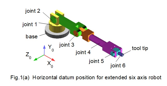
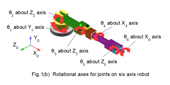
Figs.1(a) and (b) below shows the robot model with six revolute joints used in this tutorial. This model is similar to one used in previous tutorials for forward kinematics, but in this model there are no offsets between joints. Also, the rotational axes of joints 4, 5 and 6 intersect to provide a spherical wrist configuration for these joints. This arrangement simplifies the analytical method for inverse kinematics presented below.
X0, Y0 and Z0 are the real world co-ordinates of the robot base. The datum pose for the robot is a horizontal extension aligned with the X0 axis. All co-ordinate frames and rotations of joints are in accordance with the right hand rule. Thus counter-clockwise rotations are positive and clockwise rotations negative
Geometric solution for inverse kinematics
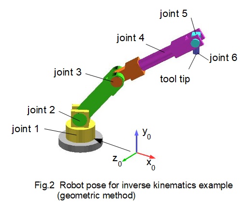
The basis for this example, originally drawn in CAD, is the pose shown above in Fig.2. The known co-ordinates of the origin of frame 5 relative to the origin of the base frame* are (in unspecified length units):
- x5 = 695
- y5 = 781
- z5 = - 401
*In previous tutorials these real world co-ordinates would be designated by a twin suffix x50, y50, z50. In this application we omit the 0 suffix for simplicity.
The tool tip is 110 units vertically below the origin of frame 5. In this configuration joint 4 and joint 6 do not rotate. Consequently joint angle θ5 is determined by joint angles θ2 and θ3. In effect, this configuration has three degrees of freedom.
Figs.3(a) and 3(b) below illustrate the geometry of the robot in the specified configuration. Note that the "elbow" at joint 3 in Fig.3(b) is in the up position. The inverse kinematic problem is to find joint angles θ1, θ2, θ3 and θ5.
Directions of rotation of joints 2, 3 and 5 illustrated in Fig.3(b) are determined from the horizontal datum position.
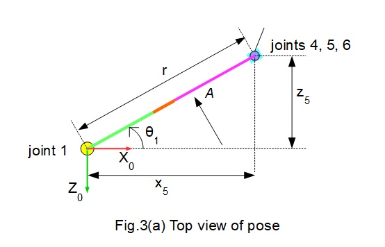
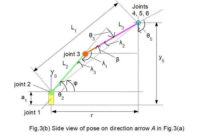
To find θ1
From Fig.3(a): θ1 = tan-1(z5 / x5) = tan-1(401/ 695): gives θ1 = 29.98°. Rotation is +ve (counter-clockwise) with the Y0 axis coming out the page on Fig.3(a).
To find θ2
From Fig.3(a): θ2 = (φ + λ3)
Also from Fig.3(a): r = z5 / sin θ1 = (401) / sin (29.98°) = 802
From the robot model: a1 = 160
From Fig.3(b): tan-1φ = tan-1(y5 - a1) / r) = tan-1(621 / 802) gives: φ = 37.74°
Also: (L1)2 = r2 + (y5 - a1)2 = (802)2 + (781 - 160)2
gives L1 = √[(802)2 + (621)2 ] = 1014
From the robot model: L2 = 400, L3 = 630
Using the law of cosines for triangle with sides L1, L2, L3 and internal angles λ1, λ2, λ3 gives:
(L3)2 = (L1)2 + (L2)2 - 2L1.L2.cos λ3
Thus θ2 = (φ + λ3) = (37.74° + 12.47°)
gives θ2 = 50.21° Rotation is +ve (counter-clockwise) with the Z0 axis coming out the page on Fig.3(b).
To find θ3
Using the law of cosines for triangle with sides L1, L2, L3 and internal angles λ1, λ2, λ3 gives:
(L1)2 = (L2)2 + (L3)2 - 2L2.L3.cos λ1
giving: θ3 = (180° - λ1 ) = (180° - 159.66°)
Thus θ3 = - 20.34° Rotation is -ve (clockwise) with the Z0 axis coming out the page on Fig.3(b)
To find θ5
From Fig.3(b): θ5 = (90° + β)
Also from Fig.3(b) β = (θ2 - θ3) = (50.21° - 20.34°) = 29.87°
Giving θ5 = (90° + 29.87°)
Thus θ5 = 119.87° Rotation is -ve (clockwise) with the Z0 axis coming out the page on Fig.3(b).
Alternative solution for θ2, θ3, and θ5
The above solution for joint angles θ2, θ3, and θ5 is not unique. Fig.3(c) below illustrates another pose providing the same tool tip co-ordinates where elbow joint 3 points down.
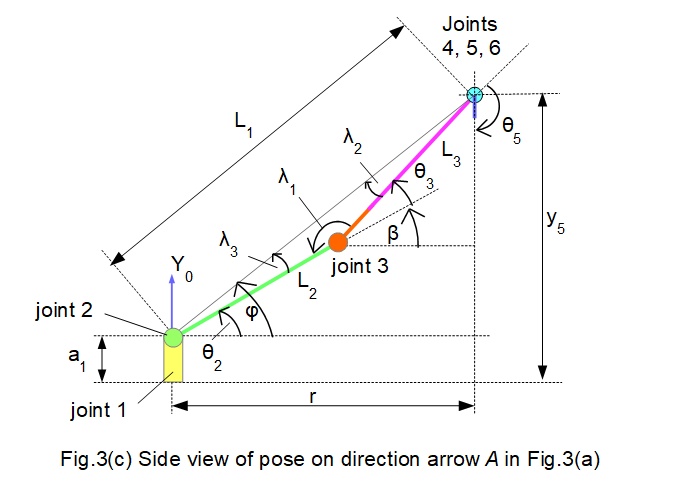
In the elbow down configuration angles are computed as follows (elbow up configuration in brackets).
θ2 = 25.27° +ve (50.21° +ve)
θ3 = 20.34° +ve (20.34° -ve)
θ5 = 119.87° -ve (135.61° -ve)
Consideration of offsets
Other variable aspects of the robot configuration, such as offsets between links, introduce multiple inverse kinematic solutions. The robot model in the examples above has no offsets but consider Fig.4 below where links between joints are offset.
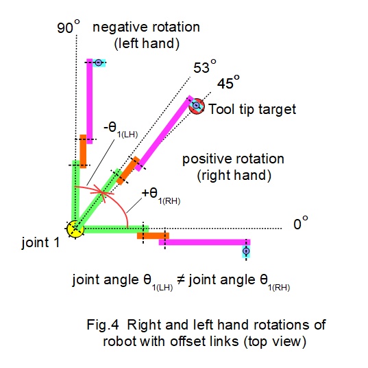
When revolute joint 1 rotates towards the mid-way angular target point from opposite directions with clockwise or counter-clockwise rotations the joint rotations θ1 are not the same. As a consequence inverse kinematics must define the direction of rotation, normally stated as right hand (counter-clockwise) or left hand (clockwise). In this example rotations to a mid-way target point from starting points 90° apart are θ1(RH) = 53° and θ1(LH) = 37°
Analytic solution for inverse kinematics
The analytic method described below considers an inverse kinematics solution for a six axis robot in two parts.
- Find a geometric solution for joint angles θ1, θ2 and θ3. For this example we apply the results from the geometric method outlined above for θ1, θ2 and θ3. We then derive the rotational transformation matrix R03 (see previous tutorial) using these values.
- The second part requires joints 4, 5 and 6 to be in a spherical wrist configuration (see above). Because of this, rotation matrix R36 alone defines transformations from co-ordinate frame 6 to co-ordinate frame 3. The elements of R36 are expressed in terms of sine and cosine functions of joint angles θ4, θ5 and θ6. Note that the pose of joints 4, 5, and 6 in this example are not the same as applied in the previous example,specifically joints 4 and 6 are rotated.
We also specify the orientation of the co-ordinate frame for joint 6 in the specified pose which determines the rotational transformation matrix R06 from frame 6 to the base frame.
The method is based on the following clever piece of linear algebra:
R06 = R03 • R36
multiply both sides by (R03)-1 (the inverse matrix of R03)
gives (R03)-1 • R06 = (R03)-1 • R03 • R36
and as (R03)-1 • R03 = I (the identity matrix) it follows:
R36 = (R03)-1 • R06.
This relationship is the basis of the procedure outlined below to resolve joint angles θ4, θ5 and θ6 where we compute (R03)-1 • R06 and use the equivalence with known matrix R36 to solve for θ4, θ5 and θ6.
Worked example of analytic method
We will work through this procedure using joint angles θ1, θ2 and θ3 from the previous worked example (elbow up configuration). For convenience joint angles are rounded to:
- θ1 = 30.0° (+ve)
- θ2 = 50.0° (+ve)
- θ3 = 20.0° (-ve)
Note that joint angles θ4, θ5 and θ6 are different from the joint angles applied in the previous example.
Step 1 - derive rotation matrix R03
R01 is rotation of +30° about the Y axis; R12 is rotation of +50° about the Z axis; R23 is rotation of -20° about the Z axis;
The inverse of a rotation matrix is its transpose, thus:
Step 2 - derive rotation matrix R06
Fig.5 below shows the horizontal datum position for the robot model as shown in Fig.1(b). Co-ordinates X0, Y0, Z0 represent the real world co-ordinate frame of the robot base.
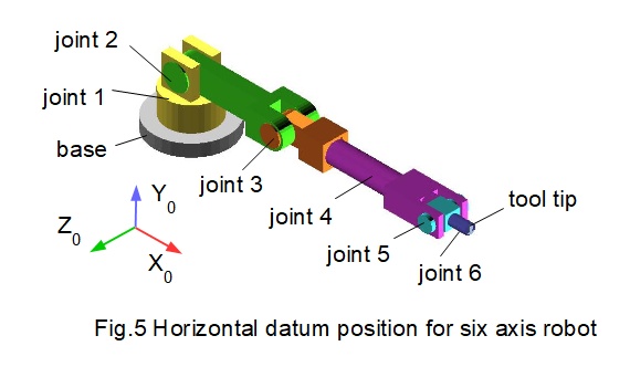
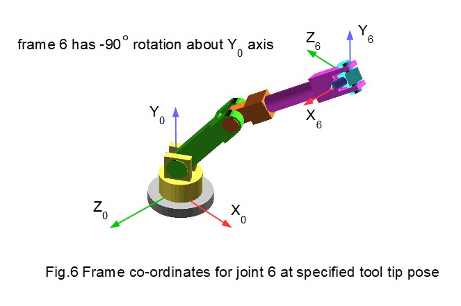
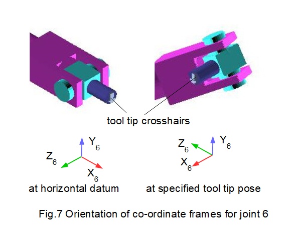
Fig.6 below shows the specified tool tip pose with the co-ordinate system for frame 6. For simplicity the transformation of frame 6 is a single (clockwise) rotation of -90° about the Y0 axis. Fig.7 below provides a more detailed view of the tool tip at the extremity of joint 6 in datum and specified pose conditions.
In a previous tutorial we found the rotational transformation matrix Ry(θ) about the Y axis to be:
which for θ = -90° gives:
Step 3 - compute rotation matrix R36
Step 4 - derive rotation matrix R36 from first principles
Firstly, note that:
- R34 is rotation of θ4 about the X axis
- R45 is rotation of θ5 about the Z axis
- R56 is rotation of θ6 about the X axis
Using rotational transformation matrices Rx(θ), Ry(θ) Rz(θ)
This operation is not entirely straightforward since multiple solutions are possible for each element.
First consider the element r11 (row 1, column 1).
Gives: cosθ5 = - 0.433
There are two possible solutions: θ5 = (i) cos-1(-0.433) = 115.7° or (ii) cos-1(-0.433) = -115.7°
Choose θ5 = -115.7° giving sinθ5 = - 0.901
Next consider element r12 (row 1, column 2)
Gives: - (sinθ5.cosθ6) = 0.5
Giving cosθ6 = - 0.5 / (- 0.901) = 0.555
Thus θ6 = (i) cos-1(0.555) = 56.3° or (ii) cos-1(0.555) = - 56.3°
Choose θ6 = 56.3° giving sinθ6 = 0.832
As a check compute element r13 (row1, column 3)
sinθ5.sinθ6 = (- 0.901).(0.832) = - 0.75 (correct)
θ6 = - 56.3° would be incorrect as sin( - 56.3°) is -ve, making r13 = +0.75
Next consider element r21 (row 2, column 1) = cosθ4.sinθ5
Gives: cosθ4 = 0.25 / ( - 0.901) = - 0.277
Thus θ4 = cos-1(- 0.277) = (i) 106.1° or (ii) cos-1(- 0.277) = - 106.1°
Choose θ4 = - 106.1° giving sinθ4 = - 0.961
As a check compute element r31 (row 3, column 1)
sinθ4.sinθ5 = (- 0.961) (- 0.901) = 0.866 (correct)
θ4 = 106.1° would be incorrect as sin(106.1°) is +ve, making r31 = -0.866
Thus the complete solution for rotation angles to effect the specified robot pose is:
| θ1 | +30.0° |
| θ2 | +50.0° |
| θ3 | -20.0° |
| θ4 | +106.1° |
| θ5 | -115.7° |
| θ6 | +56.3° |
Calculations of matrix elements r22, r23, r32 and r33 provide additional checks to validate this solution.
It can be shown that a valid solution also occurs with θ5 = + 115.7°
the resulting joint angles are:
| θ4 | +73.9° |
| θ5 | +115.7° |
| θ6 | -123.7° |
This completes the short series of tutorials on kinematics of robot manipulators.
Reurn to: Robotics content
I welcome feedback at: