In the first tutorial of this series concerning slider and crank mechanisms we firstly found from geometry an expression for displacement x of the slider as a function of crank angle θ and the ratio n (= L/R) and then differentiated with respect to time to obtain expressions for velocity and linear acceleration also as functions of θ and n.
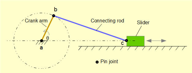
This analysis gave the required information for the slider but not the velocity and acceleration of the connecting rod, the motion of which is a combination of translational and rotational motion. This information can be obtained from velocity and acceleration diagrams. We explain these methods in this tutorial.
Firstly we review the general principles and techniques.
Velocity and acceleration diagrams
Velocity and acceleration diagrams are drawn to scale beginning with known values. Unknown values are then measured directly from the completed diagrams. It is also possible to obtain unknown values from the geometry of the diagrams and we adopt this approach below. (In the next tutorial we obtain the equivalent information directly from vector equations).
A key point when constructing velocity and acceleration diagrams is the distinction between absolute and relative quantities. Consider the velocity diagrams below which represent, say, two pin joints in a mechanism designated a and b. Arrows va and vb represent direction and magnitude of the absolute velocities of points a and b respectively relative to point o which indicates a "ground point" in a common frame of reference.
To create the velocity diagrams, va and vb are connected at their common reference point o and the diagram closed by a third arrow. In (i) the arrow direction represents the relative velocity vb/a meaning the velocity of point b relative to point a. In (ii) the arrow va/b represents the velocity of point a relative to point b.
Construction of a velocity diagram is similar to, but not exactly the same, as a conventional vector diagram shown below. In both cases the magnitude and direction of the resulting velocities are identical.
In (i) vector va is subtracted from vector vb giving the resultant vector vb/a which represents the velocity of point b relative to the velocity of point a. In (ii) vector vb is subtracted from vector va giving the resultant vector va/b which represents the velocity of point a relative to the velocity of point b.
Acceleration diagrams are constructed in a similar way to velocity diagrams bearing in mind that directions of velocity and acceleration for a point are not necessarily the same. Acceleration diagrams must also take into account that rotational motion of any point always has a radial component of acceleration directed towards the centre of rotation and a tangential component of acceleration when the point is subject to angular acceleration. The diagram below shows an acceleration diagram for the crank pin of a rotating crank arm.
In this diagram point A rotates about point O with angular acceleration α. The diagram represents a snapshot for a specific crank angle.
- aAr is the radial (centripetal) acceleration of point A relative to point O with direction from A towards O resulting from angular velocity ω.
- aAt is the tangential acceleration of point A relative to point O resulting from angular acceleration α.
- aA is the resultant acceleration of point A relative to point O.
Note that point O has two slightly different interpretations in the above depending on context. In one respect point O is the centre of rotation of the crank arm AO. In a more general context it represents a ground frame of reference.
In this example the acceleration diagram is the same as a vector diagram as all accelerations are relative to a single point O. As we shall see below this is not the case in an acceleration diagram for the complete crank mechanism.
Plane motion of a rigid body
When we examine the motion of the crank arm and connecting rod in a crank mechanism we are dealing with the kinematics of rigid bodies moving in a two dimensional plane. Classic theory approaches this as a combination of a longitudinal translation and a rotation represented in the example below.
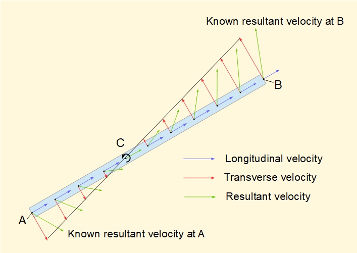
The diagram is a snapshot at one instant of velocity vectors at multiple points along the longitudinal axis of a rigid bar moving in a two dimensional plane. The longitudinal component of velocity at all points along this axis must have the same magnitude, otherwise the body would be expanding or contracting. If the absolute velocities at two points on the axis are known (in this example end points A and B) the corresponding transverse velocities perpendicular to the axis at points A and B define a pure rotational motion with centre of rotation on the longitudinal axis at point C*. This principle applies to any arbitrary line on a rigid plane body. We choose the longitudinal axis here simply for convenience.
* The point C defined here must not be confused with the instantaneous centre of rotation or velocity pole described below although as we shall see the two points are related. I adopt the description centre of rotation on the longitudinal axis on the basis that for any practical example this axis is clearly defined.
Note also that the magnitude of the rotational velocity for the centre of rotation on the longitudinal axis derived from this construction is the same whatever arbitrary line is taken for the longitudinal axis on the rigid body.
Instantaneous centre of rotation (velocity pole)
It follows from the principle of combined translational and rotational motion of a rigid body that there will be a point in the plane of motion where the tangential velocity arising from rotation is equal and opposite to the longitudinal velocity. This point of zero velocity must therefore be a centre of rotation for that instant, with every point in the body being in pure rotation around this point. The point is called the instantaneous centre of rotation or velocity pole and is illustrated in the diagram below. Note that the velocity pole does not necessarily lie on the body itself.
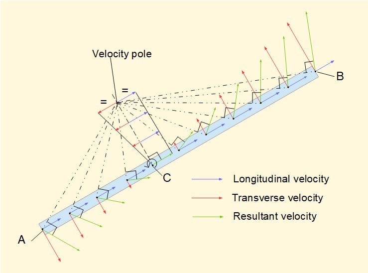
The velocity pole can be found in two ways.
- An axis is extended perpendicular to the longitudinal axis on the body through the centre of rotation on the longitudinal axis C. The notional longitudinal velocity (blue vector) is a constant at all positions on this perpendicular axis. The notional tangential velocity arising from rotation of the body (red vector) is also perpendicular to this axis but in the opposite direction and varies in magnitude. The point on this perpendicular axis where longitudinal and tangential velocities are of equal magnitude and thus cancel is the velocity pole.
- If directions of the absolute (resultant) velocities of two points on the body are known, lines perpendicular to these directions can be drawn from the respective points. The point of intersection of these perpendicular lines is the velocity pole. This is a simple and useful construction as we shall shortly see. The diagram above clearly shows how the absolute velocity of each point on the body (green vector) is tangential to a line from the velocity pole, indicating pure rotation about the velocity pole at that instant.
Velocity diagram for the slider and crank mechanism
We now construct a velocity diagram for the crank mechanism below based on a crank angle θ = 50°. The angle between the connecting rod and the horizontal axis is designated φ which we use in subsequent calculations. Dimensions and displacements are in metres.
The velocity diagram has three components:
- velocity of point A relative to O (ground) designated vA/O
- velocity of point B relative to point A designated vB/A
- velocity of point B relative to O (ground) designated vB/O
We know the following:
- The line of action of vA/O is perpendicular to the crank arm with magnitude ω.(OA) = (2π).(1) = 2π. m/s. The crank arm rotates in an counter-clockwise direction which determines the direction of vA/O
- Assuming the connecting rod is rigid the motion of point B relative to point A must be purely rotational. Thus the line of action of vB/A is perpendicular to AB.
- The motion of slider point B is constrained on a horizontal plane which defines the line of action of vB/O
The diagram below shows the lines of action of these velocities.
We now construct the velocity diagram. Firstly, calculate the magnitude of vA/O and draw the arrow to scale along the line of action. The head of the arrow represents point A relative to ground point O at the tail. Now draw the line of action of vB/A through point A and the line of action of vB/O through point O. The point of intersection of these two lines determines the magnitude and direction of vB/A and vB/O.
The completed velocity diagram is shown below. Note that the directions of vB/A and vB/O are resolved by this construction, the head of the arrow representing the velocity at that point relative to the point at the tail.
Values scaled from well drawn velocity diagrams are sufficiently accurate for practical purposes. Alternatively, velocities can be calculated directly from the diagram.
Firstly, we calculate angle φ previously mentioned:
Using the law of sines for triangle ABO:
Show angle φ on the velocity diagram with the horizontal axis and the axis of the connecting rod extended to intersect at point P.
It is now a reasonably simple matter to find sides AB and BO of triangle ABO given we know AO = vA/O = 2π m/s and angle φ = 14.79°
From triangle AOP angle PAO = 180° - (140° + 14.79°) = 25.21°
Thus in triangle ABO angle BAO = (90° - 25.21°) = 64.79°
and angle ABO = 180° - (40° + 64.79°) = 75.21°
gives BO = vB/O = 5.88 m/s
This is the identical value for the velocity of the slider for crank angle θ = 50° obtained in the previous tutorial from differentiation with respect to time, viz.
Correspondingly we calculate vA/B as follows:
gives AB = vB/A = 4.18 m/s
We use this result to find the rotational velocity ωAB of the connecting rod of length 3 m at the instant where the crank angle is 50°.
Velocity pole of the connecting rod
The diagram below shows the construction to find the velocity pole (instantaneous centre of rotation) of the connecting rod in our example mechanism where the crank angle = 50°.
Construction of the velocity pole diagram is very straightforward. Firstly, rod AB is drawn to scale at the correct angular position. In this case we know the directions of velocities vA/O and vB/O thus the velocity pole P is the intersection of lines perpendicular to these directions extended from points A and B.
Bearing in mind that the velocity pole represents the centre of pure rotational motion of the rod the rotational velocity of the rod ωAB is found by determining length AP, which is the radius of rotation for point A. We know from above that vA/O = 6.28 m/s. Thus ωAB = 6.28/AP and correspondingly by determining length BP from the diagram velocity vB/O = ωAB.BP.
AP and BP can be easily calculated, noting that we already know angle φ on the diagram
and AB = 3 m.
confirming the values of ωAB and vB/O derived from the velocity diagram in the previous section.
Centre of rotation on the longitudinal axis
We derive the centre of rotation on the longitudinal axis of the connecting rod directly from the velocity pole diagram. Single subscripts indicate absolute velocities at points on the rod.
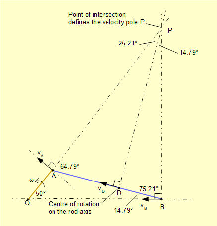
The line PD perpendicular to AB at point D extended through the velocity pole P is the radius of rotation of point D on the longitudinal axis of the rod. Thus the direction of velocity vector vD must align exactly with the longitudinal axis. Point D is the instantaneous centre of rotation on this axis and is the only point on the axis that has no transverse component of velocity.
We calculate vD with reference to the diagram as follows.
As previously calculated AP = 4.51 m
5.68 m/s is the longitudinal component of velocity at every point on the rod axis. We can check this is the case at point B where we know vB = 5.88 m/s along the horizontal axis.

Acceleration diagram for the slider and crank mechanism
The acceleration diagram for the example mechanism has the components listed as below. Lines of action of these accelerations are shown in the following diagram.
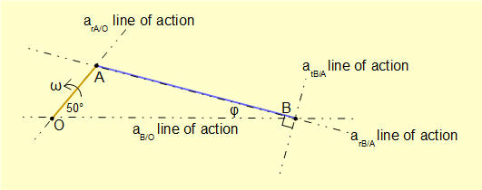
- Point A has centripetal acceleration designated arA/O acting radially along the axis of the crank arm towards its centre of rotation point O, which is also the ground reference point for the diagram. Because the crank arm rotates with constant angular velocity ω there is no tangential component of acceleration at point A. In our example arA/O = ω2.(AO) = (2π)2.(1) = 39.44 m/s2
- Point B has centripetal acceleration relative to point A designated arB/A acting radially along the axis of the connecting rod towards point A which is the centre of rotation in this case. In our example mechanism arB/A = ω2.(AB) = (1.39)2(3) = 5.80 m/s2
- We know the rotational velocity of the connecting rod ωAB is not constant and thus has angular acceleration αAB Consequently point B has a tangential acceleration relative to point A designated atAB with a line of action perpendicular to the rod. Magnitude and direction on the line of action are not known.
- Point B has acceleration relative to point O designated aB/O acting horizontally. Magnitude and direction on the line of action are not known.
We now construct the acceleration diagram, beginning with the known quantities.
Firstly, draw aA/O from an arbitrary ground point O to a point designated A on its line of action with direction from point A to point O shown on the physical diagram for the mechanism at θ = 50° (see above). It is important to note that the relative positions of A and O on the acceleration diagram are opposite to the positions on the physical diagram.
Next, draw arB/A on its line of action from point A to a point designated B/ noting the direction of this centripetal acceleration is towards its centre of rotation which in this case is from point B to point A on the physical diagram. Knowing that tangential acceleration at point B relative to point A also exists we designated this point B/, considered a part-way point between point A and point B.
Now draw the line of action of atB/A through point B/ cutting the line of action of aB/O drawn through ground point O. The intersection of these lines determines point B. atB/A is drawn from point B/ to point B and aB/O is drawn from point O to point B. The completed acceleration diagram is shown below.
Values of aB/O and atB/A obtained from a scaled diagram are satisfactory for practical purposes. However. as we did for the velocity diagram we can calculate the value of aB/O from the geometry of the diagram and compare with the value obtained previously derived from differentiation with respect to time in a previous tutorial.
The calculation is slightly more involved than for the velocity diagram. We know all angles in triangles PBO and PB/A and we know lengths OA and AB/. We then find side AP in triangle PB/A which gives side OP = OA + AP in triangle PBO from which we find side OB. The calculation gives
aB/O = 23.4 m/s2 which corresponds to the value previously obtained.
From these triangles we also calculate atB/A = 29.72 m/s2. From this value we determine the angular acceleration of the connecting rod αBA from the relation atB/A = (AB).αBA where AB = 3 m giving αBA = 9.91 rad/s2.
We will use this acceleration diagram in a future tutorial concerning inertia forces.
Next: Crank mechanism kinematics - vector equations
I welcome feedback at: