Next: Applying the steady-flow energy equation
I welcome feedback at:
In the first two tutorials in this series we introduced the First Law of Thermodynamics. We derived energy equations for closed systems with specified characteristics, recognising in certain cases differences between reversible and irreversible processes.
In this tutorial we consider flow processes in open systems and derive the thermodynamic steady-flow energy equation.
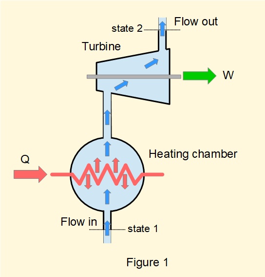
Figure 1 illustrates a generic flow process in an open system. The boundary of the system is denoted by bold lines with entry and exit points for fluid flow. In this arrangement heat \(Q\) is supplied from the surroundings to a heating chamber (for example, a steam boiler) and work \(W\) delivered from a turbine.
The steady-flow energy equation is based on the following assumptions.
The model used to derive the steady-flow energy equation is illustrated in Figure 2.
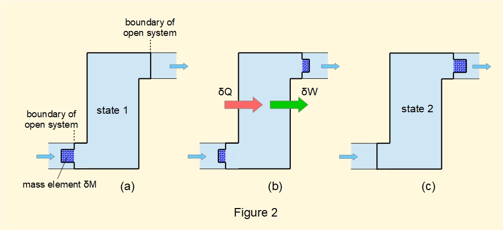
The model considers a hypothetical closed system incorporating the fluid volume in the open system and an element of fluid of mass \(\delta{M}\). Figure 2(a) shows the closed system in state 1 with \(\delta{M}\) immediately adjacent to the entry point of the system.
In Figure 2(b) we visualise \(\delta{M}\) partially entering the open system and simultaneously partially leaving at the exit point. During this transition quantities of heat \(\delta{Q}\) and work \(\delta{W}\) are transferred to and from the system.
Figure 2(c) shows the closed system in state 2 where \(\delta{M}\) leaves the open system at a position immediately adjacent to the exit point of the system.
We now consider changes in thermodynamic and mechanical properties of fluid in this closed system during the transition of \(\delta{M}\) between entry point 1 and exit point 2 located respectively at height \(z_1\) and \(z_2\) above a reference level.
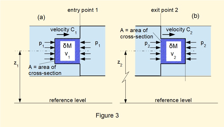
Figure 3(a) shows mass element \(\delta{M}\) about to enter the flow system at point 1. The energy of \(\delta{M}\) has three components:
Thus the total energy of element \(\delta{M}\) is: \(u_1 + \frac {1}{2}\delta {M}.{C^2_1} + \delta{M}.g.{z_1}\)
and assuming uniform properties within \(\delta{M}\) its total energy can be expressed as:
\(\delta {M}[u_1 + \frac {1}{2}{C^2_1} + g.{z_1}]\)
Designating \({E^{OS1}}\) to be the total energy in the open system at state 1 it follows that the total energy of the hypothetical closed system at state 1 is:
\({E^{OS1}} + \delta {M}[u_1 + \frac {1}{2}{C^2_1} + g.{z_1}]\)
Now referring to Figure 3(b), the total energy of \(\delta{M}\) at state 2 is: \(\delta {M}[u_2 + \frac {1}{2}{C^2_2} + g.{z_2}]\)
Designating \({E^{OS2}}\) to be the total energy in the open system at state 2 it follows that the total energy of the hypothetical closed system at state 2 is:
\({E^{OS2}} + \delta {M}[u_2 + \frac {1}{2}{C^2_2} + g.{z_2}]\)
By the assumptions stated above, the total energy in the open system is constant between states 1 and 2, thus \({E^{OS1}}\) = \({E^{OS2}}\) = \({E^{OS}}\)
Thus the respective total energies of the hypothetical closed system at states 1 and 2 can be expressed as:
At state 1: \({E^{OS}} + \delta {M}[u_1 + \frac {1}{2}{C^2_1} + g.{z_1}]\) -------- (1)
At state 2: \({E^{OS}} + \delta {M}[u_2 + \frac {1}{2}{C^2_2} + g.{z_2}]\) -------- (2)
We now consider the work associated with moving the boundaries of the hypothetical closed system at entry and exit points.
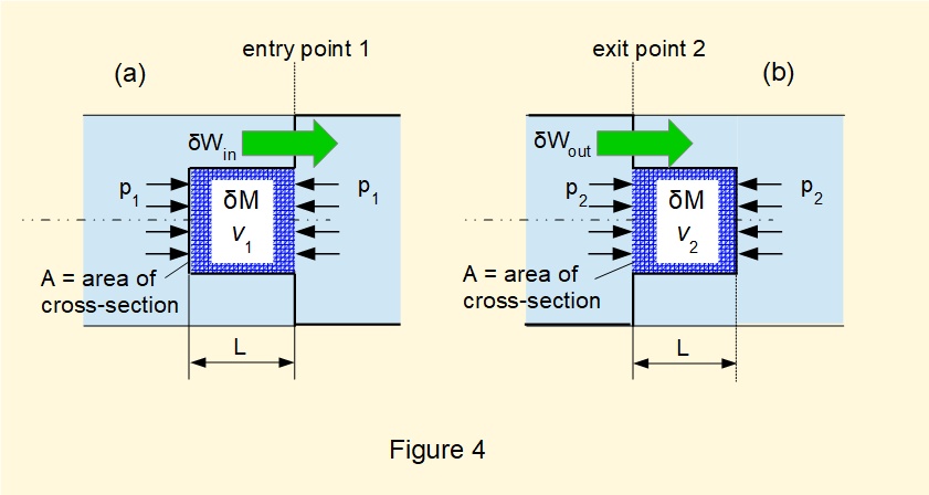
Consider in Figure 4(a) compressing element \(\delta{M}\) by pressure \(p_1\) acting on cross-section area \(A\) through distance \(L\) thus moving the boundary of the closed system inwards to the entry point of the open system.
Specific volume of \(\delta{M}\) = \(v_1\): thus volume of the element \(V_1\) = \(\delta{M}.{v_1} = A.L\)
giving work done at entry on the system: \(\delta{W_{in}} = ({p_1}.A).L = ({p_1}.A) \dfrac V A = \delta{M}.{p_1}.v_1\)
By a similar deduction in Figure 4(b), expanding element \(\delta{M}\) distance \(L\) against pressure \(p_2\) acting on cross-section area \(A\) moves the boundary of the closed system outwards from the exit point of the open system:
Specific volume of \(\delta{M}\) = \(v_2\): thus volume of the element \(V_2\) = \(\delta{M}.{v_2} = A.L\)
giving work done at exit by the system: \(\delta{W_{out}} = ({p_2}.A).L = ({p_2}.A) \dfrac V A = \delta{M}.{p_2}.v_2\)
Thus the total work done by the system to move boundaries of the hypothetical closed system is:
\(\delta{W_{out}} - \delta{W_{in}} = \delta{M}({p_2}.{v_2}-{p_1}.{v_1})\)
and the net work done by the system during the change from state 1 to state 2 is:
\(\delta{W}+\delta{M}({p_2}.{v_2}-{p_1}.{v_1})\) -------- (3)
In a previous tutorial we established from the First Law of Thermodynamics the general energy equation stating:
\(Q-W=(U+KE+PE)\)
From equations (1), (2) and (3) and the general energy equation we formulate the energy equation for an open steady-flow system as follows:
\(\delta{Q} - [\delta{W}+\delta{M}({p_2}.{v_2}-{p_1}.{v_1})] = \newline [{E^{OS}} + \delta {M}(u_2 + \frac {1}{2}{C^2_2} + g.{z_2})] - [{E^{OS}} + \delta {M}(u_1 + \frac {1}{2}{C^2_1} + g.{z_1})]\)
rearranging gives:
\(\delta{Q} - \delta{W} = \delta {M}[{u_2} + {p_2}.{v_2} + \frac {1}{2}{C^2_2} + g.{z_2}] - \delta {M}[u_1 + {p_1}.{v_1} + \frac {1}{2}{C^2_1} + g.{z_1}]\)
In the previous tutorial \((u + p.v)\) was defined as the property specific enthalpy (h) giving:
\(\delta{Q} - \delta{W} = \delta {M}[{h_2} + \frac {1}{2}{C^2_2} + g.{z_2}] - \delta {M}[{h_1} + \frac {1}{2}{C^2_1} + g.{z_1}]\) -------- (4)
Equation (4) is the steady flow energy equation for a fluid element of mass \(\delta{M}\) flowing from state 1 to state 2 in the open system. Summing elements across the entry and exit points of the system, assuming properties of the fluid are uniform across these sections gives:
\(\sum\delta{Q} - \sum\delta{W} = (\sum\delta{M})[{h_2} + \frac {1}{2}{C^2_2} + g.{z_2}] - (\sum\delta {M})[{h_1} + \frac {1}{2}{C^2_1} + g.{z_1}]\)
giving:
\(Q - W = M.[{h_2} + \frac {1}{2}{C^2_2} + g.{z_2}] - M.[{h_1} + \frac {1}{2}{C^2_1} + g.{z_1}]\) -------- (5)
where \(M\) is the mass of fluid flowing through the system in an arbitrary time interval. \(Q\) and \(W\) are amounts of heat and work transferred to or from the system during the same time interval.
Dimensions of terms on both sides of equation (5) are \(\dfrac {M{L^2}} {T^2}\) \((kJ)\)
Now divide both sides of equation (5) by \(M\) to give:
\(\dfrac {Q} {M} - \dfrac {W} {M} =({h_2}-{h_1}) + (\frac {1}{2}{C^2_2} - \frac {1}{2}{C^2_1}) + (g.{z_2} - g.{z_1})\) -------- (6)
Dimensions of terms on both sides of equation (6) are \(\dfrac {L^2} {T^2} \) \((\dfrac{kJ}{kg})\)
For engineering applications it is conventional to state equation (6) as:\({Q} - {W} =({h_2}-{h_1}) + (\frac {1}{2}{C^2_2} - \frac {1}{2}{C^2_1}) + (g.{z_2} - g.{z_1})\) -------- (7)
where \(Q\) and \(W\) are expressed in \(\Large\frac{kJ}{kg}\).
In many practical applications mass flow rate \(m\) \(\Large(\frac{kg}{s})\) is a key parameter and the steady-flow energy equation takes the form:
\(m.({Q} - {W}) = m.[({h_2}-{h_1}) + (\frac {1}{2}{C^2_2} - \frac {1}{2}{C^2_1}) + (g.{z_2} - g.{z_1})]\) -------- (7)
Units of each term in equation (7) are \(\Large\frac{kJ}{s}\) namely \(kW\).
Next: Applying the steady-flow energy equation
I welcome feedback at: