Statement of the Second Law, characteristics of the reversible Carnot cycle, establishing a thermodynamic temperature scale, deriving the property entropy from the Clausius inequality.
Statement of the Second Law
In previous tutorials we considered the First Law of Thermodynamics and its applications for non-flow and steady-flow systems. The First Law states that for a closed cycle heat engine:
\((Q_{in}-Q_{out})=W_{net}\)
The First Law does not exclude the possibility of \(Q_{out}\) being zero, thus converting all the heat absorbed by the system into work. The Second Law of Thermodynamics states that this outcome is not possible, often expressed as:
It is impossible to construct a system which will operate in a cycle, extract heat from a reservoir and do an equivalent amount of work on the surroundings.
In common with the First Law the Second Law is based on universal observation and experience.
This tutorial outlines consequences of the Second Law that lead to a definition of the useful property entropy which characterises the relationship between transfer of heat and temperature in thermodynamic processes. This classic approach begins by considering unique properties of the Carnot cycle
The Carnot cycle
In a previous tutorial we illustrated a closed cycle heat engine based on the reversible Carnot cycle as shown in Figures 1 and 2.
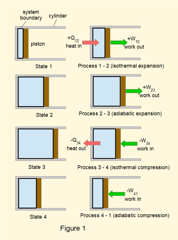
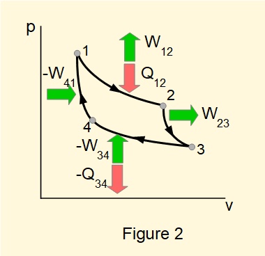
Figure 3 shows a generic form of diagram for a heat engine based on the Carnot cycle, the key feature being that heat input and output are respectively from a source and a sink at constant temperature.
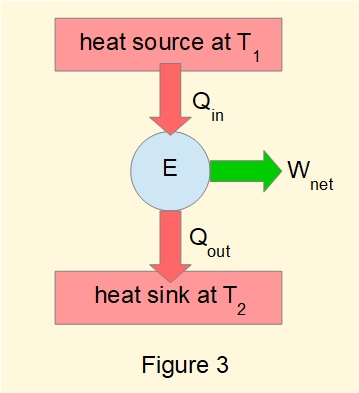
The efficiency \(\eta\) of a heat engine, when quantities of heat \(Q\) are expressed as absolute values, is defined as:
\(\large\eta=\tfrac{net\, work\, done} {heat\, supplied}=\tfrac{W_{net}}{Q_{in}}\) or \(W_{net}=\large\eta\normalsize.Q_{in}\)
If \(Q_{out}\) is the heat rejected, by the First Law: \((Q_{in}-Q_{out})=W_{net}\)
giving \(\large\eta=\tfrac{(Q_{in}-Q_{out})}{Q_{in}}\)
or \(\large\eta=1-\tfrac{Q_{out}}{Q_{in}}\) ------- (1)
These expressions for \(\eta\) apply to all heat engines with non-flow or steady-flow cycles.
A heat engine can be envisaged in terms of reversible or irreversible processes
In previous tutorials we stated the characteristics of reversible and irreversible processes in non-flow and steady-flow processes as follows:
Non-flow processes
- the system passes slowly through a sequence of equilibrium states in which all properties are uniform throughout and where changes between each state are infinitesimally small.
- infinitesimally small differences between external and internal forces apply across moving boundaries during input and output of work.
- infinitesimally small differences between internal and external temperatures apply during transfer of heat.
Steady-flow processes
- absence of viscous friction within the fluid and its interface with the system boundary*.
- infinitesimally small differences between internal and external temperatures during transfer of heat.
(* The concept of equilibrium states for steady-flow processes where fluid is in constant motion is not meaningful)
Corollaries of the Second Law with regard to reversible heat engines state:
- It is impossible to construct a heat engine operating between only two heat reservoirs which has a higher efficiency than a reversible engine operating between the same two reservoirs.
- All reversible engines operating between the same two reservoirs have the same efficiency.
It follows from these corollaries that the efficiency of a reversible engine depends only on the temperature of the reservoirs.
Derivation of a thermodynamic temperature scale
We now establish the relationship between the heat absorbed \(Q_{in}\) and heat rejected \(Q_{out}\) by a reversible heat engine operating between two reservoirs and the temperatures of the heat source and sink. By doing so, we can establish a thermodynamic temperature scale.
From equation (1):
\(\large\eta=1-\tfrac{Q_{out}}{Q_{in}}\)
Considering that \(\eta\) depends only on the temperature of the reservoirs it follows that \(\large(\tfrac{Q_{out}}{Q_{in}})\) is a function only of the temperatures of the reservoirs.
Now designate \(Q_{in}\) and \(Q_{out}\) as \(Q_0\) and \(Q\) respectively, expressed as absolute values, and consider the heat engine in Figure 4.
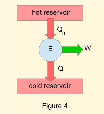
For this engine: \(\large\eta=1-\tfrac{Q}{Q_0}\) ------- (2)
where (from the above statement) \(\large(\tfrac{Q}{Q_0})\) is a function of the temperature \(T\) of the reservoirs.
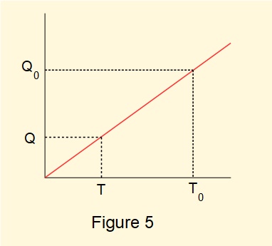
Now define a reservoir at \(T_0\) as a reference point based on a physical property of a substance and define the temperature \(T\) of any other reservoir by the linear equation:
\( T=T_0\large\tfrac{Q}{Q_0}\) --------- (3) represented in Figure 5.
We derive a temperature scale from this linear relationship as follows.
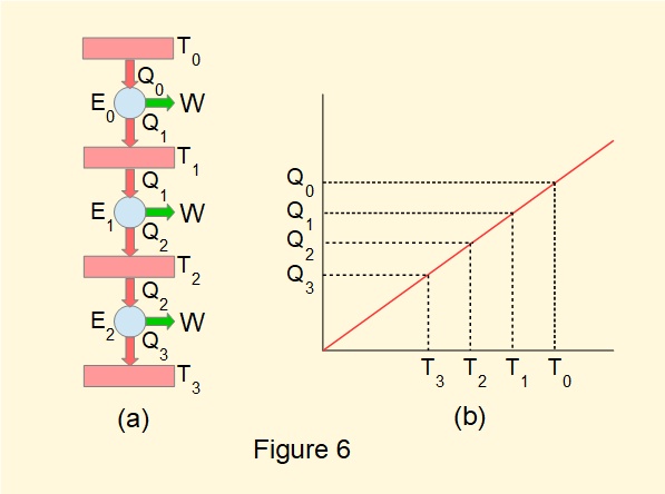
Consider Figure 6(a) illustrating a series of three heat engines designated \(E_0\), \(E_1\) and \(E_2\) each having the same work output \(W\) and heat reservoirs connected as shown. Their properties are summarised in the table below and the linear relationship between \(Q_x\) and \(T_x\) illustrated in Figure 6(b).
| Engine | T (source) | Heat in | T (sink) | Heat out | Efficiency |
|---|---|---|---|---|---|
| E0 | T0 | Q0 | T1 | Q1 | \(\eta_0\) |
| E1 | T1 | Q1 | T2 | Q2 | \(\eta_1\) |
| E2 | T2 | Q2 | T3 | Q3 | \(\eta_2\) |
Figure 6(b) shows that:
\(\large\tfrac{Q_0}{Q_1}=\tfrac{T_0}{T_1}\), \(\large\tfrac{Q_1}{Q_2}=\tfrac{T_1}{T_2}\), \(\large\tfrac{Q_2}{Q_3}=\tfrac{T_2}{T_3}\) giving \(\large\tfrac{Q_0}{T_0}=\tfrac{Q_1}{T_1}=\tfrac{Q_2}{T_2}=\tfrac{Q_3}{T_3}\) ------- (4)
It follows from equations (1) and (2) that:
\(\large\eta_0=1-\tfrac{T_1}{T_0}\), \(\large\eta_1=1-\tfrac{T_2}{T_1}\), \(\large \eta_2=1-\tfrac{T_3}{T_2}\)
giving: \(\large\eta_0=\tfrac{T_0-T_1}{T_0}\), \(\large\eta_1=\tfrac{T_1-T_2}{T_1}\), \(\large\eta_2=\tfrac{T_2-T_3}{T_2}\) ------- (5)
Recalling that \(W_{net}=\large\eta\normalsize.Q_{in}\) equal amounts of work \(W\) done by each engine are:
\( W=\eta_0.Q_0=\eta_1.Q_1=\eta_2.Q_2\) ------- (6)
combining equations (5) and (6) gives:
\(\dfrac{Q_0}{T_0}(T_0-T_1)=\dfrac{Q_1}{T_1}(T_1-T_2)=\dfrac{Q_2}{T_2}(T_2-T_3)\)
giving by equation (4):
\((T_0-T_1)=(T_1-T_2)=(T_2-T_3)\) which represents three equal intervals on a temperature scale between \(T_0\) and \(T_3\) shown in Figure 6(b).
We used three engines to establish the underlying principle but the scale can be envisaged with an infinite number of connected engines with sources at temperatures above and below the reference temperature \(T_0\).
This scale, based on the ratio \(\large(\tfrac{Q}{Q_0})\) for all reversible heat engines operating between two reservoirs, is called a thermodynamic temperature scale. Figure 6(b) shows the scale has a theoretical minimum value = 0 (absolute zero*). The internationally recognised thermodynamic temperature scale, known as the Kelvin scale (\(\degree K\)) has a reference point \(T_0\)= 273.16\(\degree K\) based on the triple point of water.
(* absolute zero temperature cannot be attained as this contravenes the Second Law, namely that a reversible heat engine cannot convert all heat input into work which from equation (5) would give \(\eta=1\) when sink temperature = 0)
Two consequences arising from the above derivation should be noted.
Firstly, as seen from equation (5) the efficiency of a reversible heat engine operating between two reservoirs increases with increasing difference between temperatures of source and sink. In practice most heat engines operate where the sink is at atmospheric temperature. Thus the theoretical maximum thermodynamic efficiency is obtained by maximising the source temperature.
Secondly, for a reversible heat engine operating between two reservoirs with \(Q_1\) from a heat source at temperature \(T_1\) and \(Q_2\) to a heat sink at temperature \(T_2\) it follows from equation (4) that:
\(\dfrac{Q_1}{T_1}=\dfrac{Q_2}{T_2}\)
The same heat engine, but irreversible, will reject more heat such that \(Q_2\) increases. Consequently:
\(\dfrac{Q_1}{T_1}<\dfrac{Q_2}{T_2}\)
Derivation of the property entropy
In this derivation we consider entropy specifically as a property of a fluid in thermodynamic systems although its application in physical sciences is much wider. We begin by considering again a cyclic heat engine, reversible or irreversible, in this instance operating with more than two reservoirs as represented in Figure 7.
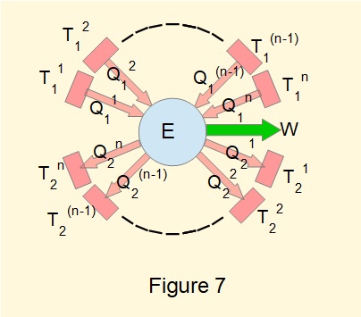
The engine has \(n\) separate sources at temperatures \(T_1^1 \rarr T_1^n\) and \(n\) corresponding sinks at temperatures \(T_2^1 \rarr T_2^n\). Respective heat inputs are \(Q_1^1 \rarr Q_1^n\) and heat outputs \(Q_2^1 \rarr Q_2^n\) for each source and sink.
We do not present it here but it can be proved from the First Law that:
\(\displaystyle\sum_1^n \dfrac{Q_1}{T_1} - \displaystyle\sum_1^n \dfrac{Q_2}{T_2} \leqslant 0 \) ------- (7)
We can interpret equation (7) in terms of algebraic quantities of \(Q\) throughout one complete cycle of the engine as:
\(\sum \dfrac{{\delta}Q}{T} \leqslant 0\) where \({\delta}Q\) represents one small element of the total \(Q\) associated with a single value of \(T\).
Taking the limiting case of \(n\) elements in Figure 7 such that \(n \rarr \infty\) gives:
\(\Large \oint \tfrac{dQ}{T} \normalsize \leqslant 0\) ---- (8) For a reversible engine it can be shown that: \(\Large \oint \tfrac{dQ}{T} \normalsize = 0\) ----- (9)
( \(\Large \oint\) in this context signifies line integration through one complete cycle from an arbitrary starting point to the same finishing point)
Equations (8) and (9) are known as the Clausius Inequality
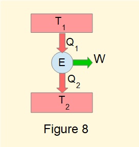
A heat engine operating between two reservoirs at constant temperatures \(T_1\) and \(T_2\) as in Figure 8 provides a particular application of the Clausius Inequality such that:
\(\Large \oint \tfrac{dQ}{T} = \tfrac{Q_1}{T_1} - \tfrac{Q_2}{T_2} \normalsize \leqslant 0\)
If the engine is reversible, from equation (4): \(\dfrac{Q_1}{T_1} = \dfrac{Q_2}{T_2}\)
giving \(\dfrac{Q_1}{T_1} - \dfrac{Q_2}{T_2} = 0\) confirming the Clausius inequality for a reversible cycle in equation (9).
If the engine is irreversible: \(\dfrac{Q_1}{T_1} - \dfrac{Q_2}{T_2} < 0\) and so \(\dfrac{Q_2}{T_2} > \dfrac{Q_1}{T_1}\)
Having established the Clausius inequality in the context of cyclic processes we now consider \(\large(\tfrac{dQ}{T})\) for processes in closed systems in terms of a corollary of the Second Law as follows:
There exists a property of a closed system such that a change in its value is equal to \(\int_1^2 \large(\tfrac{dQ}{T})\) for any reversible process undergone by the system between state 1 and state 2.
This property is called entropy denoted by \(S\) with units \(\Large\frac{kJ}{\degree K}\). Specific entropy is denoted by \(s\) with units \(\Large\tfrac{kJ}{kg \degree K}\)
The corollary stated above can be expressed as follows:
\(\large\int_1^2 (\tfrac{dQ}{T})_{rev} = \normalsize S_2-S_1\) where rev shows the relation applies only to a reversible process,
or in differential form \(dS = (\large\tfrac{dQ}{T})_{rev}\) ------- (10)
It follows that \(Q_{rev} = \large\int_1^2 \normalsize T.ds\) ------- (11)
The above equations are for positive values of \(Q\) with heat transfers from source to system. For negative values of \(Q\) with heat transfers from system to sink the sign of \(Q\) is reversed, giving:
\(\large\int_1^2 (\tfrac{dQ}{T})_{rev} = \normalsize S_1-S_2\)
Finally, we state below another corollary of the Second Law (without proof) concerning adiabatic processes:
The entropy of any closed system which is thermally insulated from the surroundings either increases, or if the process undergone by the system is reversible, remains constant.
As a property entropy is similar to internal energy in that only differences in values are used for engineering applications. For this purpose the established reference point where \(S\) is zero is the saturated liquid at the triple point