Review of entropy, applications in non-flow and steady-flow processes, internal and external entropy changes in irreversible processes
Review of entropy
In the previous tutorial we derived an expression defining the property entropy by considering transfers of heat \(Q\) at variable temperatures \(T\) in a heat engine. This definition is stated as a corollary of the Second Law of Thermodynamics as follows:
There exists a property (entropy) of a closed system such that a change in its value is equal to \(\int_1^2 \large(\tfrac{dQ}{T})\) for any reversible process undergone by the system between state 1 and state 2.
Entropy is denoted by \(S\) with units \(\Large\frac{kJ}{\degree K}\). Specific entropy is denoted by \(s\) with units \(\Large\tfrac{kJ}{kg \degree K}\)
The definition stated above can be expressed as follows where \(dQ\) is the increment of heat per unit mass:
\(\large\int_1^2 (\tfrac{dQ}{T})_{rev} = \normalsize s_2-s_1\) where rev shows the relation applies only to a reversible process,
or in differential forms: \(ds = (\large\tfrac{dQ}{T})_{rev}\) and \((dQ)_{rev}=T.ds\)
from which it follows that \(Q_{rev} = \large\int_1^2 \normalsize T.ds\)
The above relations are for positive values of \(Q\) with heat transfers from source to system. For negative values of \(Q\) with heat transfers from system to sink the sign of \(Q\) is reversed, giving:
\(\large\int_1^2 (\tfrac{dQ}{T})_{rev} = \normalsize s_1-s_2\)
Application of entropy in thermodynamic systems
In previous tutorials we considered applications of the First Law for processes in closed systems with no-flow and then for processes in open systems with steady-flow, noting that steady-flow processes may be linked to form a closed cycle. We follow the same approach to illustrate the application of entropy.
Entropy in closed non-flow applications
Previously we used \(pv\) diagrams to illustrate reversible paths for closed processes between states 1 and 2 where \(\large\int_1^2 \normalsize p.dv\) represents work \(W\) input or output from the process.
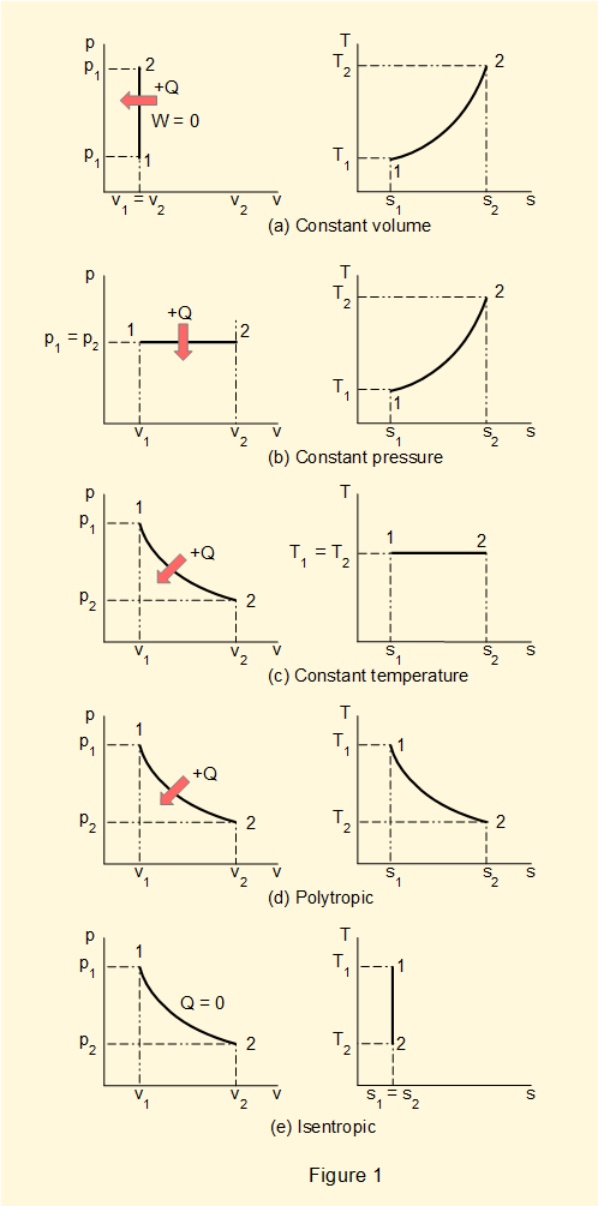
From the relation \(Q_{rev} = \large\int_1^2 \normalsize T.ds\) it follows that the area below a \(Ts\) diagram between state 1 and state 2 gives the heat \(Q\) transferred.
Figure 1(a-e) shows \(Ts\) diagrams* with corresponding \(pv\) diagrams for five reversible closed processes, namely:
- Constant volume (isochoric) with heat transfer
- Constant pressure (isobaric) with heat transfer
- Constant temperature (isothermal) with heat transfer)
- Polytropic with heat transfer
- Adiabatic (no heat transfer)**
* profiles of curves in the diagrams are indicative only
** a reversible adiabatic process is called isentropic
Application to the Carnot cycle
In a previous tutorial we presented the reversible Carnot cycle as a closed cycle comprising a sequence of four closed processes.
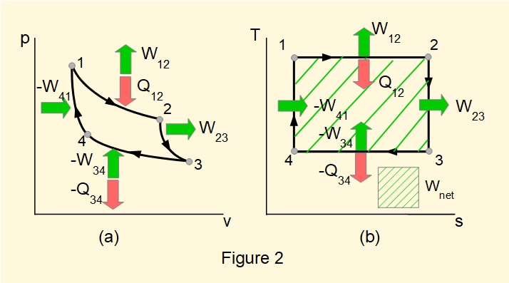
Figure 2 shows \(pv\) and \(Ts\) digrams for a reversible Carnot cycle.
- process 1-2: isothermal expansion, heat in, work out (entropy increases)
- process 2-3: isentropic expansion, work out (constant entropy)
- process 3-4: isothermal compression, heat out, work in (entropy decreases)
- isentropic compression, work in (entropy decreases)
On the \(Ts\) diagram:
\(Q_{12} = \large\int_1^2 \normalsize T.ds\) = area under 1-2 = \(Q_{in}\)
\(Q_{34} = \large\int_3^4 \normalsize T.ds\) = area under 3-4 = \(Q_{out}\)
By the First Law \((Q_{in}-Q_{out})=W_{net}\)
Thus the enclosed area on the \(Ts\) diagram represents the net work done over one reversible cycle as does the enclosed area on the \(pv\) diagram.**
(** Figures 2(a) and (b) do not have the same scale with respect to net work)
Entropy in steady-flow applications
In a previous tutorial we developed the steady-flow energy equation from an imaginary closed system reproduced in Figure 3 with additional parameters relating to entropy. The model envisages an element of mass \(\delta{m}\) progressing from entry to the open system at state 1 to exit at state 2. The boundary of the imaginary closed system incorporates \(\delta{m}\).
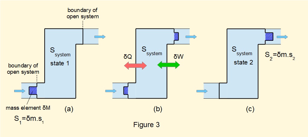
For steady-flow the total entropy inside the boundary of the open system \(S_{system}\) is constant. Entropy \(S_1\) of element \(\delta{m}\) is \(\delta{m}.s_1\) where \(s_1\) is specific entropy of the fluid about to cross the boundary of the open system at state 1. Entropy \(S_2\) of element \(\delta{m}\) is \(\delta{m}.s_2\) where \(s_2\) is specific entropy of the fluid immediately after crossing the boundary of the open system at state 2.
Now consider an adiabatic system, namely \(Q=0\).
Total entropy of the imaginary closed system at state 1 is \((\delta{m}.s_1 + S_{system})\)
Total entropy of the imaginary closed system at state 2 is \((\delta{m}.s_2 + S_{system})\)
A previously stated corollary of the Second Law declares the following:
The entropy of any closed system which is thermally insulated from the surroundings either increases, or if the process undergone by the system is reversible, remains constant.
Thus it follows that: \((\delta{m}.s_2 + S_{system})\geqslant (\delta{m}.s_1 + S_{system})\)
giving: \(\delta{m}.s_2 \geqslant \delta{m}.s_1\) and consequently \(\sum\delta{m}.s_2 \geqslant \sum\delta{m}.s_1\)
Each element \(\delta{m}\) enters and leaves the open system with identical properties at states 1 and 2 respectively such that it follows: \(\large s_2 \geqslant s_1\)
and for a reversible adiabatic (isentropic) steady-flow process: \(\large s_2 = s_1\)
This result has useful applications in steady-flow processes such as expansion through a turbine where the flow can be considered isentropic as a first approximation.
Entropy changes in irreversible processes
Irreversible processes fall into two categories, external and internal.
Internal irreversibility
The change in entropy in a process between two states equals the line integral of \(\large\tfrac{dQ}{T}\) along any reversible path between these states. The change in entropy of an irreversible process between two states cannot be determined by this integral. Generally, the path of an irreversible process is indeterminate.
We use the term entropy generated to encompass effects of viscous friction, turbulence, diffusion and other irreversible phenomena in fluids. In engineering applications process efficiency factors derived from practical tests are often applied to account for generated entropy .
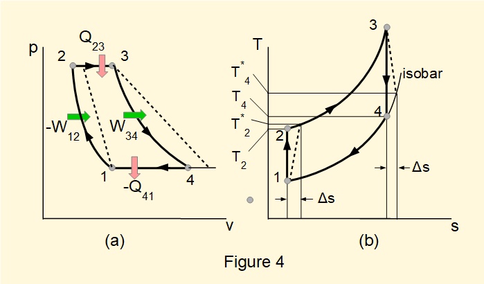
Figure 4 shows \(pv\) and \(Ts\) diagrams for a reversible closed steady-flow gas cycle, known as the Joule (or Brayton) cycle. Cooled air is compressed isentropically (stage 1-2), heated from an external source at constant pressure (stage 2-3), expanded through a turbine isentropically producing work (stage 3-4) and cooled at constant pressure with heat rejected externally (stage 4-1). A portion of the work from the turbine drives the compressor.
Irreversible processes in the compressor and turbine are shown using the conventional method of dashed (or dotted) lines. Paths between start and end points of irreversible processes are arbitrary and do not represent thermodynamic states during the process. Modified temperatures \(T^*_2\) and \(T^*_4\) and internal entropy \({\Delta}s\) generated during expansion and compression are indicated on the \(Ts\) diagram.
Internal irreversibility in turbines and compressors is accounted for by applying isentropic efficiencies defined as:
for a turbine: \(\large\eta\normalsize_T = \dfrac{W_{actual}}{W_{isen}}\) and for a compressor \(\large\eta\normalsize_C = \dfrac{W_{isen}}{W_{actual}}\)
Applying values of \(\large\eta\normalsize_T\) and \(\large\eta\normalsize_C\) based on experiment enables a reliable estimate of the state of the working fluid at exit.
External irreversibility
Change in entropy of fluid in a reversible process between two states 1 and 2 caused by transfer of heat from an external reservoir, for example stage 2-3 in Figure 4(b), is determined by
\(\large\int_1^2 (\tfrac{dQ}{T})_{rev}\). A reversible process requires an infinitesimal temperature difference between the reservoir and fluid in the system but where heat is conducted though a boundary wall there is always a temperature gradient. This creates an external irreversibility.
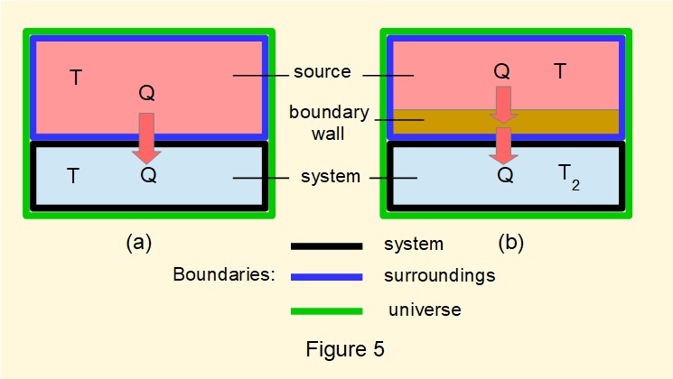
Figure 5(a) illustrates a reversible process where a quantity of heat \(Q\) is supplied from a source (reservoir) at temperature \(T\) to a system with an infinitesimal difference in temperature. The reservoir is considered to be of sufficiently large volume for temperature \(T\) to remain constant. In this arrangement we designate the reservoir as the "surroundings" and the surroundings plus the system as the "universe".
Changes in entropy are accordingly:
for the surroundings: \(\Delta S_{sur}=-(\dfrac{Q}{T})\) for the system: \(\Delta S_{sys}=+(\dfrac{Q}{T})\)
It follows that the overall change in entropy in this "universe" is: \((\Delta S_{sys}-\Delta S_{sur})=0\)
In Figure 5(b) a boundary wall is placed between the reservoir and the system such that the surroundings now comprise the reservoir and the wall. Heat \(Q\) transfers at the boundary between the reservoir and the wall at temperature \(T\) and is conducted through the wall by virtue of a temperature gradient, the temperature at the boundary between the wall and the system being \(T_2\).
Transfer of heat \(Q\) through the boundary wall occurs at a steady rate. There is no change of state of the wall during heat transfer, thus the entropy of the wall remains constant.
Changes in entropy where surroundings include the boundary wall are:
for the surroundings: \(\Delta S_{sur}=-(\dfrac{Q}{T})\) for the system: \(\Delta S_{sys}=+(\dfrac{Q}{T_2})\)
As \(T > T_2\) it follows that \((\dfrac{Q}{T_2}) > (\dfrac{Q}{T})\) and consequently \(\Delta S_{sys} > \Delta S_{sur}\).
Thus the entropy of the universe (surroundings plus system) has increased by \((\Delta S_{sys}-\Delta S_{sur})\) on account of the external irreversibility of transferring heat from a hot body to a colder body*.
(* Another statement of the Second Law (the Clausius Statement) is that it is impossible for heat to flow spontaneously from a colder to a hotter body without any external work being performed on the system)
This analysis exemplifies the axiom that the total entropy within the cosmic universe is constantly increasing.
Consequences of external irreversibility on efficiency
Consider operation of a heat engine as follows:
- heat from the engine is rejected to a sink at temperature \(T_0\)
- operating mode A has no external irreversibility: heat is transferred to the engine from surroundings at source temperature \(T_1\).
- operating mode B has external irreversibility: heat is transferred to the engine at temperature \(T_2\) from surroundings containing the same source plus a boundary wall.
From the previous analysis it follows that \(T_2 < T_1\)
In a previous tutorial we derived the following expression for the efficiency \(\large \eta\) of a heat engine in terms of the temperatures of heat in and heat out:
\(\large\eta=\Large\tfrac{T_{in}-T_{out}}{T_{in}}\)
giving for modes A and B
\(\large\eta_A=\Large\tfrac{T_1-T_0}{T_1}\) \(=1-\Large\tfrac{T_0}{T_1}\) and \(\large\eta_B=\Large\tfrac{T_2-T_0}{T_2}\) \(=1-\Large\tfrac{T_0}{T_2}\)
as \(\dfrac{T_0}{T_2} > \dfrac{T_0}{T_1}\) it follows that \(\large\eta_B < \large\eta_A\)
The maximum amounts of work that can be produced by the engine in modes A and B by a quantity of heat input Q are:
for mode A: \(Q.\large\eta_A\) for mode B: \(Q.\large\eta_B\)
Thus the amount of heat rendered unavailable to produce work for a given quantity of heat input \(Q\) on account of this external irreversibility is: \(Q(\large\eta_1-\eta_2)\)
Next: Properties of liquids and vapours
I welcome feedback at: